Regular Sturm-Liouville problems II- Second order linear ordinary differential equations and zeros of solutions

Second-order linear ordinary differential equations (ODE) stand at the heart of countless models in mathematics and physics, from the simplest harmonic oscillator to far more intricate systems with variable coefficients. While explicit closed-form solutions are sometimes available, much of their essential character can be read from a purely qualitative feature: the zeros of the solutions (the points at which they cross or touch the equilibrium line). The number, spacing, and interlacing of these zeros reveal how rapidly a solution oscillates, how its behavior changes with the coefficients, and how different solutions of the same equation relate to one another.
In the first article, I talked about the functional analysis fundamentals. In this article, I explore the basic tools for constructing and understanding such solutions, beginning with the auxiliary equation for constant-coefficient problems, the Euler-Cauchy and the power-series method for equations with variable coefficients. I then introduce Sturm’s classical comparison and separation theorems, which provide powerful, explicit-free ways to locate and compare zeros across solutions and across different equations. These ideas form the foundation for the deeper oscillation theory that will later illuminate the structure of regular Sturm-Liouville problems.
Second Order Linear ODEs

Then L[y]=f is a second-order ODE on a real interval I. We say L is linear since, for any two class C² functions \varphi, ψ, two complex numbers c₁ and c₂:

Now, let c by a point belonging to the real interval I such that a₀(c)=0, then we call c a singularity and the equation is irregular. On the other hand, if for all points x of I a₀(x) is not zero, then the equation is regular and we can let:

By the existence and uniqueness theorems, if q(x),r(x), and g(x) are continuous on I and x₀ belongs to I, then:

Solving these kind of equations requires us to identify the structure: if g(x)=0, the equation is homogeneous and there exists two linearly independent solutions y₁(x), y₂(x) on I such that the general solution is a linear combination:

If g(x) is not zero, then the equation is inhomogeneous and a particular integral yₚ shall be found (many methods) and added to the general solution:

Constant coefficient linear ODES
Consider the equation:

And let f(x)=0, when the coefficients are constants, the linear homogeneous equation admits an elegant exact solution via the auxiliary (or characteristic) equation. We simply try an exponential trial solution:

Differentiating twice and substituting immediately yields this quadratic:

The two roots λ₁, λ₂ completely determine the shape of the general solution (a linear combination of two independent basis functions). Distinct real roots give decaying or growing exponentials; a repeated root brings a factor of xe^{\lambda x}; complex conjugate roots produce the familiar damped or undamped oscillations e^{\alpha x} (\cos \beta x + \sin \beta x).
Intuitively, think of the auxiliary equation as the frequency selector for the linear operator. Because constant coefficients make the equation translation invariant (due to linearity), pure exponentials are eigenfunctions of differentiation, and the algebraic equation simply asks which growth or decay rates (frequencies) are compatible with the differential equation. This is why we obtain closed-form solutions for free particles, simple harmonic motion, uniform vibrating strings, etc.
Euler-Cauchy
For the Euler-Cauchy equations, where:

Power series
As soon as the coefficients become functions of x (the generic situation in Sturm-Louville problems coming from separation of variables in cylindrical or spherical coordinates) the exponential ansatz (solution guess) fails. There is no single λ that works for every x. The power series method (and its Frobenius extension for regular singular points) restores constructivity; we assume a solution of the form:

around an ordinary or regular singular point x₀. Substituting into the differential equation produces a recurrence relation that determines every coefficient aₙ for n greater or equal than 2 in terms of the two arbitrary constants a₀, a₁. The resulting series converges in a disk (or up to the nearest singularity), giving an analytic solution that can be continued or matched to boundary conditions.
We can found solutions to certain second order ODEs through alternative methods. If one solution is known or guessed, the second is found by a first-order equation in the unknown multipliers. For non-homogeneous problems, variation of parameters can be used. Sometimes, numerical analysis methods can also work.
Boundary conditions
A second-order linear differential equation by itself describes an entire two-parameter family of possible solutions -think of it as a broad canvas of curves that all satisfy the same local relationship between a function, its slope, and its curvature. To single out one specific solution (or a discrete set of them) that matches a concrete physical or mathematical situation, we must supply two additional pieces of information. When these constraints are imposed at the ends of the interval on which we are working, they are called boundary conditions. They tell us, for example, that the solution must take a prescribed value at each endpoint (Dirichlet conditions, such as y(a)=0 and y(b)=0), that its slope must vanish there (Neumann conditions, such as y’(a)= 0), or that a linear combination of the value and the slope must satisfy a certain relation (Robin or mixed conditions).
Intuitively, boundary conditions act like the anchors that hold the solution in place: fixed ends of a vibrating string, insulated tips of a heat-conducting rod, or an elastically supported beam. Once these anchors are fixed, the differential equation and the boundary conditions together select solutions with very particular zero distributions (certain numbers of crossings inside the interval become allowed or forbidden). In this way, boundary conditions transform the general theory of second-order equations and their zeros into precise, well-posed problems whose solutions exhibit the structured oscillatory behavior we explore in the rest of this article.
For (1) on the real closed interval I that goes from a to b, the solution may be subjected to boundary conditions at interval’s end points, taking the form of:

Generalizing:

Where:

Then, the boundary value problem (BVP) is given by equations (1), (2) and (3). If ξ = η =0 then the boundary conditions are homogeneous. If α₃=α₄=β₃=β₄=0, we say that the boundary conditions are separated. We call periodic boundary conditions to: y(a)=y(b), y’(a)=y’(b).
The Wronskian
Let f and g be two differentiable functions, the Wronskian of f and g is defined as:

The Wronskian W helps us detect independence. If you imagine the two functions as curves, W measures whether their value-and-slope pairs are pointing in linearly independent directions at each point (remember that the determinant of a 2x2 matrix tells you whether two vectors are parallel -linearly independent-).
Get Γ(z)’s stories in your inbox
Join Medium for free to get updates from this writer.
When W is nowhere zero on an interval, the two functions are linearly independent: neither is a constant multiple of the other, and together they span the entire solution space of a second-order linear equation.
For solutions of the same homogeneous equation, Abel’s identity shows that W is either zero or never zero; it can change sign only if the solutions are dependent. This fact is the hidden engine behind Sturm’s separation theorem (which I will mention and prove later): because a non-vanishing Wronskian forces the ratio y₂/y₁ to be strictly monotonic between consecutive zeros of y₁ , the second solution is compelled to cross zero exactly once in every such interval. In short, the Wronskian converts the local geometric idea of two curves not being multiples of each other into a global statement about how their zeros must alternate.


Now, regarding linear independence:

Try to prove yourself this little lemma with the definition of linear dependence.
Zeros distribution
A zero of a solution y(x) is simply a point where the graph crosses or touches the equilibrium line y=0 . For a second-order linear equation the solution is uniquely determined by its value and derivative at any single point; consequently, a non-trivial solution can have at most a simple zero (if y(x₀)=y’(x₀)=0 , uniqueness forces y is equivalent to 0).
Intuitively, picture y(x) as the transverse displacement of a vibrating string or the wave function of a quantum particle. Each zero is a node, i.e.: a quiet point that never moves. The local spacing between consecutive zeros tells us the local wavelength and therefore the local frequency or energy cost. Where the restoring coefficient is large, zeros cluster more tightly; where it weakens, the solution stretches out.
It is important to say that the number and distribution of zeros along with other qualitative features of a solution (if any) to:

are governed by the coefficients q(x) and r(x). For example, consider the BVP:

We say that a function f has an isolated zero x₀ in I if:

Using that definition, we prove the following lemma:

It is time to talk about (and prove it) the Sturm’s separation Theorem which is the precise statement that independent solutions of the same equation take turns crossing zero.


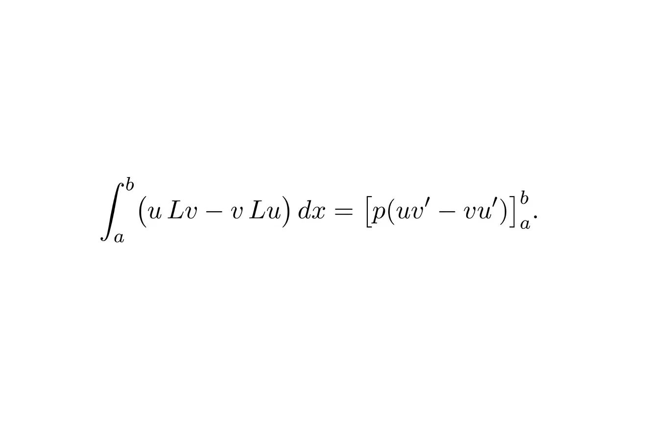
Now, to state and prove the Sturm’s comparison theorem we need the self-adjoint form of the equation (it is in the third article of this series that I’ll talk fully about the self-adjoint, do not worry about the fundamentals for now).

Since v cannot be zero, the zeros of u coincide with those of y.
While separation compares two solutions of one equation, comparison Theorem compares the oscillation rates of two different equations.

The statement of Sturm’s comparison Theorem can be reduced to: the solution of y oscillates at least as fast as that of z. Larger r means a stronger restoring force. Think of two strings with the same length and boundary conditions but different tensions or densities. The higher-tension string has nodes closer together.

Lastly, we say that a non-trivial solution for y’’+r(x)y=0. is oscillatory if it has infinite number of zeros. If r is less or equal to zero, then the solution does not oscillate. But, if:

then any solution of the equation has infinite number of zeros distributed between the zeros of any solution of y’’+k2y=0.
The tools developed in this article (the Wronskian and Abel’s identity, the precise control of zeros via Sturm’s separation and comparison theorems, the transformation that puts any second-order equation into self-adjoint form, and the role of boundary conditions in selecting solutions with definite nodal patterns) are the concrete, geometric skeleton on which the entire abstract theory of regular Sturm-Liouville operators rests.
In short, everything that feels abstract in the next articles (domains of self-adjoint operators, essential self-adjointness, discrete spectrum, eigenfunction expansions, etc.) acquires clear intuitive meaning once we have seen how zeros behave, how independent solutions take turns, and how boundary conditions turn a differential expression into a well-posed, self-adjoint boundary-value problem. The tools developed in this article (the Wronskian and Abel’s identity, the precise control of zeros via Sturm’s separation and comparison theorems, the transformation that puts any second-order equation into self-adjoint form, and the role of boundary conditions in selecting solutions with definite nodal patterns) are the concrete, geometric skeleton on which the entire abstract theory of regular Sturm-Liouville operators rests.
In short, everything that feels abstract in the next articles (domains of self-adjoint operators, essential self-adjointness, discrete spectrum, eigenfunction expansions, etc.) acquires clear intuitive meaning once we have seen how zeros behave, how independent solutions take turns, and how boundary conditions turn a differential expression into a well-posed, self-adjoint boundary-value problem.
Recommended books
Al-Gwaiz, M. A. (2008). Sturm — Liouville theory and its applications. Springer.
Bear, H. S. (1999). Differential equations: A concise course. Dover Publications.
Graef, J. R., Henderson, J., Kong, L., & Liu, S. X. (2018). Ordinary differential equations and boundary value problems: Volume I. Advanced ordinary differential equations. World Scientific.