Transformers vs. ARIMA: Do More Complex Models Produce Better Forecasts?

Time-series forecasting problems can look very different depending on the data you’re working with. Financial prices are noisy and hard to predict, electricity demand follows strong daily and weekly patterns tied to human activity, and airline passenger data layers a pronounced trend on top of recurring seasonality. A model that handles one of these well won’t necessarily do as well on another.
That’s why I’m skeptical of the idea that there’s one best forecasting tool, or that newer automatically means better. It’s also the question behind this project: do transformer-based models actually outperform simpler statistical methods across different kinds of time series, or does the extra complexity only pay off in certain settings?
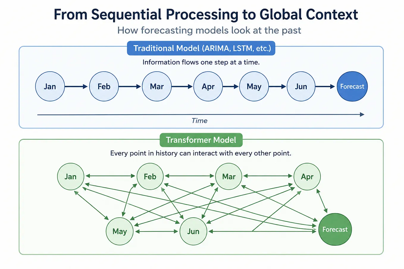
Transformers reshaped natural language processing, and they’re showing up more and more in forecasting too. Their ability to capture complex relationships and long-range dependencies makes them appealing for time-series problems. But classical models like ARIMA haven’t gone anywhere, and for good reason: they’re transparent, relatively inexpensive to run, and built on statistical ideas that have been tested for decades.
I compared both approaches under the same forecasting framework instead of assuming either one should win.
Three Different Forecasting Problems
To make the comparison meaningful, I tested the models against three datasets that behave very differently:
- SPY — a noisy financial series where short-term price movements are notoriously difficult to predict.
- Airline passengers — a classic monthly series with a clear upward trend riding on top of strong annual seasonality.
- Electricity demand — an hourly series shaped by recurring daily and weekly patterns.
Testing across all three tells you more than any single dataset could. A win for transformers only on highly structured series would say one thing; holding up even on something as noisy as SPY would say something more surprising; and classical models keeping pace across the board would suggest the extra complexity isn’t buying much.
What I care about isn’t just which model wins overall — it’s when the added complexity actually earns its keep.
Methodology
A model comparison is only as good as the evaluation behind it. I built the experiment around walk-forward evaluation, which means that at every forecast date, each model only gets access to information that would actually have been available at that point in time. It makes a forecast, I compare that forecast with what happened next, and then the process moves forward.
That is closer to how forecasting works in practice than a single train-test split, and it reduces the chance that the results are driven by one unusually lucky or unlucky test period.
I also froze the dataset splits, forecast dates, horizons, preprocessing rules, and evaluation metrics before comparing the final models. Once the experiment was set, I didn’t change those rules because one model happened to perform poorly.
Datasets and Forecast Horizon
The three datasets operate on very different timescales, so I chose horizons that were meaningful for each problem rather than forcing them into the same definition.

The electricity series contained 24 missing hourly observations. I restored the regular hourly index and interpolated those gaps; all 24 occurred before the 2025 evaluation period.
Every model was evaluated on the same frozen forecast origins within each dataset, so the errors are directly comparable.
Classical and Transformer Models
The classical side starts with a Naive persistence forecast, which simply uses the most recent observed value as the prediction for the future. That sounds almost too simple to matter, but it is a surprisingly difficult benchmark to beat on persistent series , especially financial prices.
I then use an ARIMA-family model selected using training data only. The exact specification varies by dataset because the structure varies by dataset:
- SPY uses ARIMA(0,1,2) with drift
- Airline passengers uses a seasonal log-SARIMA model
- Electricity uses a log-transformed weekly-difference ARIMA model.
Model selection never uses observations from the evaluation period.
The transformer side includes two very different approaches:
- Chronos-2, a pretrained foundation model used zero-shot
- PatchTST, a supervised transformer trained from scratch separately at every forecast origin.
I’ll explain those differences in more intuitive terms in the next section.
Measuring Forecast Performance
I use several complementary measures of forecast error:
- RMSE gives more weight to large errors.
- MAE measures the average absolute miss.
- MASE scales errors relative to a simple historical benchmark, making it easier to interpret performance across different types of series.
- Directional accuracy asks whether the model correctly predicts whether the series moves up or down from the forecast origin.
For MASE, the scaling value is recomputed at every forecast origin using historical data only. Airline uses a 12-month seasonal benchmark, electricity uses a 168-hour weekly benchmark, and SPY uses a nonseasonal benchmark.
I also monitor model fitting and training diagnostics. That matters because a forecast can look perfectly valid even when the underlying optimization did not behave as intended. In the ARIMA runs, for example, I tracked convergence at every origin and used a conservative retry procedure when needed rather than silently dropping failed fits. For the neural-network model, I checked training behavior, finite predictions, and data leakage throughout the walk-forward process.
Finally, for SPY and electricity , where there are enough forecast origins , I use paired forecast-comparison tests to check whether apparent differences in error are likely to be more than random variation. I also adjust those tests for the fact that I’m making multiple comparisons. With only 13 airline forecast origins, I treat those results primarily as descriptive rather than making strong statistical claims.
The full model specifications, optimizer handling, training parameters, and statistical-test implementation are better suited to the technical project documentation, so I’ll keep the focus here on what the models are doing and what the results tell us.
Models Compared
The experiment includes four models that represent very different forecasting philosophies, chosen to compare approaches that make increasingly ambitious assumptions about what information and complexity are needed to produce a useful forecast.
Naive Forecast
The simplest model in the experiment is the Naive forecast, and its rule is about as basic as it gets: the best guess for tomorrow is today’s value.
If SPY closes at 500 today, the Naive model forecasts 500 for the next period. The same logic applies to airline passengers and electricity demand , whatever the most recent number was, that becomes the forecast.
That might sound too simple to be useful, but it’s an important benchmark. A lot of real-world data doesn’t change dramatically from one period to the next, so tomorrow often looks a lot like today. A complicated model shouldn’t get credit just for producing a forecast. It has to beat a rule that requires almost no modeling at all.
So the Naive model sets up the first real question in this project: can the more sophisticated models actually do better than assuming things stay the same?
ARIMA and SARIMA
The next step up is the ARIMA family of models. Unlike the Naive forecast, ARIMA actually looks at patterns in the history of the series. It uses recent changes and relationships between past observations to estimate where the series may be headed. For data with strong seasonal patterns, there’s a seasonal extension called SARIMA.
These models are built specifically for time-series data, and they give you a structured way to capture things like:
- persistence,
- trends,
- short-term relationships,
- and recurring seasonal patterns.
The exact model varies by dataset because each series behaves differently. SPY gets an ARIMA model aimed at short-term dynamics. Airline passengers gets a seasonal version that explicitly accounts for the strong yearly pattern. For electricity demand, the model first accounts for the strong weekly repetition in usage before modeling what remains.
Together, these provide a strong classical benchmark: considerably more sophisticated than Naive, but still relatively transparent and built on well-understood statistical relationships.
Chronos-2
Chronos-2 takes a very different approach. Instead of building a new model specifically for each dataset, it’s a pretrained time-series foundation model, conceptually similar to how a large language model is trained on huge amounts of text before it’s asked to work with a new piece of writing.
Chronos has already been trained on a broad collection of time-series data, so I give it the historical observations for SPY, airline passengers, or electricity demand and ask it to forecast what comes next.
I run Chronos zero-shot. It is never retrained or fine-tuned on any of my three datasets. It sees the historical series and produces a forecast using what it learned during its original pretraining.
That’s a genuinely different question from the one ARIMA and PatchTST are answering. Instead of asking whether you can train a model that performs well on this specific dataset, zero-shot forecasting asks something closer to: can a large pretrained model recognize useful patterns in a time series it has never been trained on, with no dataset-specific training at all?
If the answer is yes, that’s a meaningful advantage. It means you may be able to get strong forecasts without building and training a separate model for every new problem.
PatchTST
PatchTST is also transformer-based, but it takes the opposite approach from Chronos. Instead of arriving with knowledge learned from a broad collection of time series, PatchTST is trained specifically on the dataset it is being asked to forecast.
Rather than looking at every observation independently, it breaks the history into small chunks, or patches, and learns relationships between those chunks while preserving their chronological order. That lets the model learn how patterns evolve through time rather than treating the series as an unordered collection of values.
For every forecast origin in the experiment, I train a brand-new PatchTST model using only the historical data available at that point. That makes it a more traditional supervised machine-learning approach: give the model examples from this specific dataset and let it learn which patterns help it forecast.
The contrast with Chronos is worth emphasizing. Chronos arrives with knowledge from large-scale pretraining but never trains on my datasets. PatchTST has no outside knowledge going in, but it gets to learn directly from each individual dataset.
Comparing the two helps separate two ideas that often get lumped together under the word transformer: the value of the architecture itself and the value of large-scale pretraining.
Four Different Forecasting Strategies
At a high level, the four models represent four increasingly different ways of thinking about forecasting:

That range matters once you get to the results. A win for the most complex model would suggest the added sophistication is worth the cost. A strong showing from something as simple as ARIMA would suggest the opposite: that complexity on its own isn’t buying much. And there’s a more specific version of that question sitting between Chronos and PatchTST — if the pretrained model outperforms the one trained from scratch, that points to the advantage coming from pretraining itself, not just from using a transformer architecture in the first place.
Results
SPY: Complexity Doesn’t Help Much in a Noisy Market
SPY turned out to be the clearest example of a forecasting problem where more sophisticated models didn’t produce better results.
At the shortest horizon, the Naive forecast was the best model. Its one-step RMSE was 4.36, compared with 4.37 for ARIMA — in practical terms, a negligible difference. That isn’t especially surprising. For a highly liquid financial series like SPY, the most recent observed price is already a very strong short-term benchmark. Daily price movements are noisy, and new information gets priced in quickly, which makes consistent one-step-ahead improvements difficult.
At longer horizons, ARIMA did pull slightly ahead. At five steps, it reduced RMSE by about 1% relative to Naive. At 20 steps, that improvement grew to roughly 3.3%.

Those gains are interesting, but they shouldn’t be overstated. When I formally compared the forecast errors, ARIMA’s improvements over Naive at the 5- and 20-step horizons didn’t remain statistically significant after adjusting for the multiple comparisons in the experiment. ARIMA produced slightly smaller errors on average, but the evidence isn’t strong enough to say it consistently beats simply using the most recent SPY value.
The Zero-Shot Transformer Struggled
Chronos-2 performed noticeably worse than both classical approaches. At one step ahead, its RMSE was about 68% higher than Naive’s. That gap narrowed as the horizon increased, but Chronos still didn’t beat either classical benchmark. At 20 steps, its RMSE was 20.95, compared with 20.37 for Naive and 19.70 for ARIMA.
The statistical comparison tells a similar story. ARIMA significantly outperformed Chronos at the 1- and 5-step horizons after adjustment; at 20 steps, the difference was no longer statistically significant. Chronos became more competitive as the horizon grew, but there’s no evidence here that its pretrained architecture provided a meaningful advantage on SPY.
Training a Transformer From Scratch Performed Much Worse
PatchTST produced the weakest results by a wide margin. Its one-step RMSE was 37.38, compared with roughly 4.36 for Naive and 4.37 for ARIMA. Even at 20 steps, its RMSE remained above 41.
This wasn’t a failure of training. All 380 origin-specific PatchTST models trained successfully, produced finite forecasts, and passed the leakage and validation checks. The problem was predictive performance: the model simply didn’t uncover useful structure that the simpler models were missing.
That doesn’t mean PatchTST is inherently a poor forecasting model. It means that under this fixed experiment, training a modest transformer from scratch on SPY’s history didn’t help. It’s a useful illustration of a broader theme in the project: a more flexible model can’t invent predictable structure where very little may exist in the first place.
Direction Was Difficult Too
Get Eric Clower’s stories in your inbox
Join Medium for free to get updates from this writer.
The directional results tell the same general story. ARIMA achieved about 50% directional accuracy at one step, 63% at five steps, and 70% at 20 steps. Chronos-2 came in at 47%, 41%, and 44%, while PatchTST stayed below 46% across all three horizons.
ARIMA’s longer-horizon numbers are interesting, but I’d interpret them cautiously. Financial prices tend to drift upward over long periods, so predicting direction over longer intervals can become easier even when precise point forecasts remain difficult. The takeaway isn’t that ARIMA “predicts the market.” It’s that neither transformer approach produced a clear improvement over relatively simple classical benchmarks.
What SPY Tells Us
SPY is a good counterexample to the idea that a more advanced architecture should automatically win. The simplest model came out on top at one step, ARIMA gained only modest ground at longer horizons, Chronos-2 never caught either classical benchmark, and PatchTST added substantial complexity while producing dramatically larger errors.
For this series, the limiting factor looks less like model sophistication and more like the amount of predictable signal available in the data.
Airline Passengers: Strong Seasonal Structure Favors Classical Modeling
The airline passenger data produced a very different result from SPY.
Here, the series has strong, visible structure: a long-term upward trend combined with a repeating annual seasonal pattern. That gives forecasting models much more consistent information to work with.
The best-performing model at all three forecast horizons was seasonal ARIMA. At one month ahead, SARIMA reduced RMSE by roughly 79% relative to Naive. At three months, the reduction was about 81%. Even at a full 12-month horizon, SARIMA still cut RMSE by nearly 60%.

That’s one of the real strengths of classical seasonal models: when a series has stable, recurring structure, explicitly modeling that structure can pay off enormously.
Chronos-2 Was Competitive, but Not Best
Chronos-2 beat the Naive forecast by a wide margin at every horizon: roughly 71% lower RMSE at one month, 77% lower at three months, and 49% lower at 12 months.
That’s a strong showing for a model that received no dataset-specific training. Chronos still recognized enough structure in the series to substantially outperform simple persistence.
It didn’t beat SARIMA, though. Compared with the seasonal model, Chronos’s RMSE was about 38% higher at one month, 23% higher at three months, and 24% higher at 12 months.
That makes airline passengers a good example of a pretrained model being genuinely capable while still falling short of a model explicitly designed around the series’ own seasonal behavior.
PatchTST Struggled With the Small Sample
PatchTST performed poorly here. Its one-month RMSE was 87.74, and it remained substantially worse than both SARIMA and Chronos at every horizon.
Again, this wasn’t a numerical stability problem. The issue was the amount of data available. At the start of the evaluation period, the model had only 120 monthly observations to work with. Once those were converted into supervised training windows, each PatchTST fit had only 49 to 61 actual training examples — a tiny sample for a neural network with thousands of parameters.
Most airline PatchTST fits also ran all the way to the maximum number of training epochs instead of stopping early, and the forecasts tended to stay within a narrow range. The model struggled to extrapolate the continuing upward trend in passenger counts.
This is where the difference between the two transformer approaches becomes especially clear. Chronos arrived with patterns learned during large-scale pretraining. PatchTST had to learn everything from scratch from one small monthly dataset. On data this limited, that difference mattered.
Directional Accuracy Looks Strong, but Needs Context
Both SARIMA and Chronos posted very high directional accuracy on the airline series, about 92% at one month and 100% at both three and 12 months.
Those numbers look impressive, but the series has a strong upward trend, so correctly predicting that a future value will be higher than the current value is much easier here than it is for something noisy like SPY. Directional accuracy therefore carries less information than the error metrics. What matters more is how closely each model predicts the magnitude of future passenger levels, and on that measure SARIMA remains clearly strongest.
What Airline Passengers Tell Us
The airline results show that newer models don’t automatically replace well-specified classical methods. Chronos-2 does surprisingly well with no dataset-specific training, but seasonal ARIMA does better because its structure closely matches what’s actually happening in the data.
PatchTST, meanwhile, shows how difficult it can be to train a flexible neural network from scratch when the historical sample is small. For a short, strongly seasonal series like this one, explicitly modeling the structure you already know is there remains extremely effective.
Electricity Demand: Where the Pretrained Transformer Stands Out
Electricity demand produced the strongest result for Chronos-2 and the clearest example in the experiment of a pretrained transformer adding real forecasting value.
Unlike SPY, electricity demand has strong recurring structure: usage shifts by hour of day, day of week, and broader seasonal patterns. But unlike the airline series, that structure is high-frequency and more complex. That combination appears to suit Chronos particularly well.
Chronos had the lowest RMSE at all three horizons. At one hour ahead, it came in about 46% lower than Naive and 41% lower than ARIMA — a genuinely substantial improvement. At 24 hours, the advantage over Naive narrowed to about 1%, but Chronos remained nearly 50% better than ARIMA. At 168 hours, a full week out, Chronos reduced RMSE by roughly 14% relative to both classical models.

ARIMA Worked Well at One Hour, but Broke Down at 24 Hours
ARIMA’s performance is especially interesting because it varied sharply by horizon. At one hour ahead, it improved meaningfully on Naive, with RMSE falling from 1,036.52 to 940.77. At 24 hours, however, RMSE jumped to 3,102.45 — nearly double the Naive result. By 168 hours, ARIMA and Naive were essentially tied again.
That pattern suggests the weekly-difference ARIMA specification captured useful very short-term behavior, but that structure didn’t translate into an accurate day-ahead forecast. It doesn’t mean ARIMA is generally poor for electricity forecasting. It means this particular training-selected specification did not perform consistently across horizons , and because the experiment was frozen, I did not retune it after seeing that result.
Chronos Was More Consistent Across Horizons
Chronos wasn’t just better at the shortest horizon. It stayed competitive or best as the forecast window widened.
What makes that notable is that Chronos received no electricity-specific training. It was given only the historical demand series available at each forecast origin and asked to predict what came next. A pretrained model picked up on useful recurring structure in hourly demand without being explicitly given hour-of-day or day-of-week variables and without any fine-tuning on this dataset.
The experiment can’t tell you exactly which learned patterns Chronos relied on, but it does show that whatever it learned during pretraining transferred well to this problem.
The Statistical Evidence Is Strongest at Shorter Horizons
The formal forecast-comparison tests support the one-hour result most clearly. After correcting for multiple comparisons, Chronos significantly outperformed both ARIMA and Naive at one hour, and it also significantly outperformed ARIMA at 24 hours.
At 168 hours, the raw error differences still favored Chronos, but they did not remain statistically significant after adjustment. The one-week forecast looks better on average, but the evidence is weaker that the advantage is consistent enough to generalize beyond this particular evaluation window.
PatchTST Again Failed to Add Value
PatchTST didn’t match Chronos here either. At one hour, its RMSE was 2,742.15 — more than four times Chronos’s error. At 24 hours it did manage to beat ARIMA, but it still trailed both Chronos and Naive. At one week, its RMSE was almost identical to the classical benchmarks and still about 16% worse than Chronos.
That makes this result especially useful because electricity is the dataset where a transformer clearly can work well, as Chronos demonstrates. PatchTST shows that using a transformer architecture on its own isn’t enough. The pretrained model succeeds, while the one trained from scratch does not.
That contrast points toward the advantage coming less from the architecture by itself and more from the broad time-series patterns Chronos learned before it ever saw this dataset.
What Electricity Demand Tells Us
Electricity is the strongest evidence in this experiment that modern pretrained forecasting models can add real value. Chronos clearly improves the one-hour forecast, stays highly competitive at 24 hours, and produces the lowest RMSE at one week.
At the same time, PatchTST’s weak showing means the takeaway isn’t “transformers beat classical models.” The takeaway is narrower and more useful: a pretrained transformer can be highly effective when what it learned transfers well to the structure of the problem in front of it.
Does the Added Complexity Pay Off?
Forecast accuracy is only part of the decision when choosing a forecasting model. A more complex model might produce lower error, but that improvement has to be weighed against the time it takes to train, the compute it needs, and the effort required to maintain it.
In this experiment, the four approaches had very different computational requirements.

Chronos-2 is particularly interesting because it shifts most of the training cost outside the experiment. The model was already pretrained before I used it; once loaded, I only needed to provide the historical series and run inference.
PatchTST is the opposite. Because it was trained from scratch at every forecast origin, the experiment required 477 separate training runs, totaling roughly 3,208 seconds — or about 53 minutes — of CPU training time. Despite that additional cost, PatchTST didn’t win a single dataset-and-horizon comparison on RMSE, MAE, or MASE.
More Computation Did Not Mean Better Forecasts
SPY is the clearest example. PatchTST required an average of about 8 seconds of training per forecast origin, and its forecasts still came out substantially worse than the nearly costless Naive benchmark. The average recorded per-origin times were about 2.16 seconds for ARIMA fitting and forecasting, 0.56 seconds for Chronos-2 inference, and 7.99 seconds for PatchTST training.
Airline passengers followed a similar pattern. PatchTST trained quickly because the dataset was small, but that same lack of data made it difficult for the model to learn a useful forecasting relationship. Seasonal SARIMA stayed substantially more accurate.
Electricity told a different story. Chronos was both the most accurate model and relatively inexpensive to apply. It averaged about 0.64 seconds of inference per forecast origin, compared with nearly 29 seconds for repeated ARIMA fitting and forecasting — roughly a 45-fold difference in the recorded per-origin runtime for this experiment.
That isn’t a universal speed benchmark: Chronos timing excludes its one-time model-loading cost, while the ARIMA timing includes repeated estimation. But from the perspective of this walk-forward exercise, Chronos was both more accurate and substantially faster to apply on electricity.
Pretraining Changes the Cost Equation
The contrast between Chronos and PatchTST says something important about how foundation models change the economics of forecasting.
Both are transformer-based, but their costs land in very different places. PatchTST has to learn from scratch on each dataset. Chronos arrives with patterns learned during large-scale pretraining and applies that knowledge directly to a new series.
The original pretraining of Chronos was, of course, computationally expensive; that cost doesn’t disappear. But from the perspective of someone using an already-trained model, the relevant cost is mostly inference rather than training a new neural network from scratch.
That distinction mattered here. Chronos produced the best electricity forecasts without any dataset-specific training, while PatchTST required hundreds of independent training runs and still couldn’t outperform Chronos on any dataset or horizon.
Complexity Is Worth It Only When It Adds Value
Complexity should be treated as a cost that has to earn its place in a forecasting system.
It didn’t earn its place for SPY, where Naive and ARIMA stayed stronger than either transformer approach. For airline passengers, explicit seasonal modeling remained the best solution. For electricity demand, though, the pretrained Chronos model delivered real improvements without PatchTST’s repeated training cost.
None of this means complex models should be avoided. It means complexity needs to be justified by measurable improvement on the actual problem in front of you.
Sometimes the simplest benchmark is genuinely hard to beat. Sometimes a well-specified classical model already captures the structure in the data. And sometimes a pretrained foundation model earns its extra sophistication by delivering real predictive value.
What matters isn’t how advanced a model is. It’s whether the added complexity earns its keep.
Limitations and Statistical Caution
The results are useful, but worth reading within the limits of how the experiment was built. A few things are worth keeping in mind:

What This Adds Up To
Taken together, these limitations narrow the claim rather than undermine it. The experiment does not show that one model class is universally best. It shows that across these three carefully controlled forecasting problems, complexity by itself was not enough to guarantee better forecasts.
Conclusion
No single model won this experiment. What determined the winner was how well a model’s strengths matched the structure of the problem in front of it.
- For SPY, the simplest approaches were hardest to beat. Naive won at the shortest horizon, and neither transformer added meaningful value on a series this noisy.
- For airline passengers, strong seasonality favored the model built specifically to represent it: seasonal ARIMA beat both transformers at every horizon.
- For electricity demand, Chronos-2 produced the strongest forecasts at all three horizons with no dataset-specific training — the clearest case in the experiment where a pretrained transformer beat the classical benchmarks outright.
- PatchTST, trained from scratch at every forecast origin, never won a single comparison despite the additional computational cost.
Across all nine dataset-and-horizon comparisons, ARIMA or SARIMA had the lowest error in five, Chronos-2 in three, Naive in one, and PatchTST in none. The same winner counts held for RMSE, MAE, and MASE.
That’s not a record that supports the idea that modern forecasting models have simply replaced classical ones.
The better lesson is that forecasting is still a model-selection problem. A classical model can be very hard to beat when a series has real, interpretable seasonal structure. Added flexibility buys you little when there isn’t much predictable signal to find. And a pretrained foundation model can deliver strong forecasts with no dataset-specific training when what it learned transfers well to the problem you give it.
So instead of starting with Which model is the most advanced?, I’d start with a plainer question:
What’s the simplest model that performs well enough for this specific problem?
Whatever complexity you add after that has to earn its place. How well it does that depends on the data, the forecast horizon, the available training history, and what it costs you to get the forecast wrong.
Better forecasting isn’t about picking the newest model. It’s about matching the model to the problem.
Replication materials available here.