Distributed Systems

Ddp

Parameter Server

Pytorch

Grpcio

DISTRIBUTED TRAINING: WHAT I LEARNED BUILDING A PYTORCH TRAINING SYSTEM FROM SCRATCH

Funboy Ea

6 min read

·

Feb 23, 2026

--

Listen

Share

More often than not, I wake up with an undying thirst for knowledge. On a faithful morning weeks ago, I woke up wanting to understand what actually happens under the hood when large models are trained across multiple machines. Since I’m currently GPU poor, I could only experiment with small DNN models, in a later time, I will work on extending this to support transformer models.

The result is DistributedTraining, a PyTorch playground that implements and compares three training strategies: a single-node baseline, a Parameter Server (sync and async), and DDP with gradient compression and fault tolerance layered in.

This post is a walkthrough of what I learned.

The Scenario

Before anything technical, here’s a mental model I’ll reuse throughout.

Imagine a classroom of students sitting for an exam. But instead of testing knowledge, they’re building it. Each student is responsible for studying a different chapter of a massive textbook. After studying their chapter, each student writes down what they learned (gradients), and those notes need to be combined into one shared understanding that everyone agrees on.

That shared understanding is our model.

The obvious challenge is combining everyone’s notes efficiently, keeping things consistent, and handling a situation where a student falls asleep mid-exam.

There are three ways to run this classroom.

Single Student (Baseline): One student reads the entire textbook alone.

Teacher and Students (Parameter Server): A teacher holds the authoritative textbook. Students each study a chapter and hand their notes to the teacher. The teacher updates the book and hands updated copies back. Repeat.

Students Teaching Each Other (DDP): There is no teacher. Every student has their own copy of the book. After studying, they pass notes around the room in a ring until everyone has seen everyone else’s notes and can update their book identically.

Keep this analogy in mind as we move forward.

The Foundation: Protobuf and gRPC

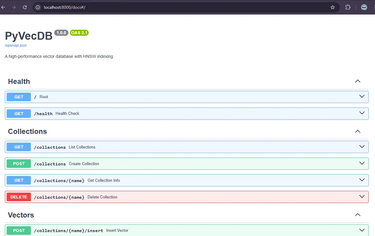
In a parameter server architecture, before any training happens, the system needs a shared language, a contract that defines exactly what messages can be exchanged between machines/workers. This is what distributed.proto provides.

Protocol Buffers (Protobuf) define structured data. Message types are defined once and can be serialized and deserialized efficiently across languages.

In this system, the core message types are:

• TensorProto — the package format for sending any tensor: raw binary data, shape like [32, 10], dtype like "float32", and a requires_grad flag.
• GradientMessage — what a worker sends after a backward pass: worker_id, a map of parameter names to tensors, whether compression was used, if yes, the compression type, and the training step.
• ParameterMessage — what the server sends back: model weights plus a version counter that increments with every update.
• HeartbeatMessage — a worker saying “I’m alive”: worker_id, timestamp, and current epoch.
• WorkerAssignment — the server assigning a worker its rank and world_size.

On top of these, two services are defined:

• ParameterServerService — exposes SendGradients, GetParameters, and RegisterWorker.
• CoordinatorService — exposes SendHeartbeat and ReportMetrics.

gRPC runs on top of these definitions. It auto-generates server-side and client-side classes from the proto file. When a worker calls SendGradients, gRPC handles serialization, transmission, and deserialization transparently. Strong typing ensures errors are caught at system boundaries, not buried deep in training logic.

Serialization: Packaging Tensors for the Network

The serialization.py layer sits between PyTorch and gRPC. Its job is to convert tensors into network-transmittable formats and back.

The pipeline works in five layers:

1. Dtype conversion — torch.float32 ↔ "float32".
2. Binary serialization — torch.save() converts tensors to raw bytes; torch.load() reconstructs them. Tensors are detached and moved to CPU first.
3. Dictionary payloads — metadata (shape, dtype, requires_grad) is added alongside binary data for validation.
4. State dictionary support — applies the above transformation to every tensor in a model state_dict.
5. Protobuf integration — converts dictionary payloads into TensorProto messages ready for gRPC transmission.

The design choice is separation. The serialization layer knows nothing about gRPC. The gRPC layer knows nothing about PyTorch.

The Baseline: Single-Node Training

BaselineTrainer serves as the control group.

It trains a SimpleCNN using a standard PyTorch loop: forward pass, loss computation, backward pass, optimizer step, repeat.

The network consists of:

• Two convolution layers (32 and 64 filters),
• Max pooling after each,
• Two fully connected layers (128 → 10),
• Dropout at 0.5.

It automatically adapts to MNIST, Fashion-MNIST, and CIFAR-10 input shapes.

The purpose is simple: establish a performance and accuracy baseline.

One student. One textbook.

The Parameter Server

This is where distributed complexity begins.

The server holds the authoritative model and aggregates gradients.

Worker Registration

Workers call RegisterWorker. The server assigns a rank and confirms world_size, ensuring stable cluster identity.

Async Mode

Workers send gradients via SendGradients. The server immediately applies them and increments the version counter.

This is fast but gradients may be applied to slightly stale model versions.

Sync Mode

The server buffers gradients from all workers. Once every worker has submitted gradients for a step, it averages them and applies the update.

Consistent but is limited by the slowest worker.

Model Fetching

Workers call GetParameters after each update. A lock prevents mid-update reads. Workers use the returned version to check model freshness.

Compression Handling

The server transparently detects compression_type and decompresses gradients before aggregation.

Thread-safe locks ensure safe concurrent access.

The Workers

Workers perform the actual learning.

Each worker holds:

• A model copy,
• A unique data shard,
• gRPC connections,
• Optional compression settings.

Training Loop

1. Forward pass
2. loss.backward()
3. Collect gradients
4. Compress (if enabled)
5. Send gradients
6. Receive updated parameters
7. Log metrics

Gradient time, communication time, and compression ratio are logged via TensorBoard.

Heartbeat

A background thread sends periodic heartbeat messages to the coordinator for failure detection.

Data Sharding

The dataset is partitioned into non-overlapping shards. Each epoch reshuffles deterministically for reproducibility.

Gradient Compression

Two interchangeable compressors implement a shared interface.

QuantizationCompressor

Reduces float32 tensors to int8 (≈4× compression).

Steps:

• Compute min and max
• Compute scale: (max - min) / 255
• Quantize: round((x - min) / scale) - 128
• Store quantized values with min and max metadata
• Decompress via inverse mapping

Some precision is lost, but convergence is often barely affected in practice.

TopKCompressor

Keeps only the top-k gradients by absolute magnitude.

Steps:

• Flatten tensor
• Compute k = ceil(numel * compression_ratio)
• Store top-k indices and values
• Zero-fill on decompression

With compression_ratio = 0.01, you send 1% of gradients, potentially 10×–100× compression depending on indexing overhead.

Practical Insight

Compression helps most when communication time dominates compute time. At small scale, CPU overhead from compression can cancel out bandwidth savings. It becomes clearly beneficial only when gradients are large and the network is a real bottleneck.

The Coordinator

The coordinator manages worker lifecycle, monitoring, and recovery.

Responsibilities

• Start workers
• Monitor heartbeats
• Detect failures
• Trigger recovery
• Aggregate metrics

Failure Recovery

When a worker fails:

1. Save a system checkpoint
2. Reassign data shards temporarily
3. Restart worker from checkpoint
4. Restore original shard partitioning

This imitates simplified fault-tolerance mechanisms found in frameworks like Ray and Horovod.

DDP: Ring AllReduce

Pytorch’s DDP removes the central server entirely.

Each worker holds a full model copy. After loss.backward(), gradient synchronization happens automatically via Ring AllReduce. This helps with abstracting what goes on behind the scenes.

Workers:

• Pass gradients around in a logical ring,
• Accumulate partial sums,
• Divide by world_size.

Every model stays perfectly synchronized.

No bottleneck node. No single point of failure.

However, workers must remain in lockstep. One slow worker slows everyone.

Retry Logic and Resilience

retry_with_exponential_backoff() wraps network operations.

On failure:

• Wait
• Retry with exponential delay
• Add jitter to avoid thundering herd effects, in simpler terms, introducing a random delay to operations, to prevent a large number of requests from hitting a system simultaneously and overwhelming it.

In distributed systems, transient network failures are expected, not exceptional.

Observability

TensorBoard logging tracks:

• Loss
• Accuracy
• Throughput
• Per-worker compute time
• Communication time
• Compression ratio

Performance comparison reports generate JSON summaries across baseline, PS, and DDP runs.

Key Experimental Findings

At small scale, overhead matters more than expected.

PS aggregation and gRPC round-trips consume significant time.

DDP scales more cleanly due to decentralized communication.

Async PS trades consistency for flexibility.

Sync PS trades speed for reproducibility.

Compression only provides gains when communication is the dominant cost.

Conclusion

Observing synchronous mode stall on a slow worker, or asynchronous mode drift due to stale gradients, illustrated theoretical trade-offs in practice.

This project reminded me of a fundamental principle of engineering: performance optimization is context-dependent, and more often than not, every architectural decision introduces measurable trade-offs.

The full implementation, configs, Docker setup, compression modules, coordinator, and reporting scripts — is available in the GitHub repository.