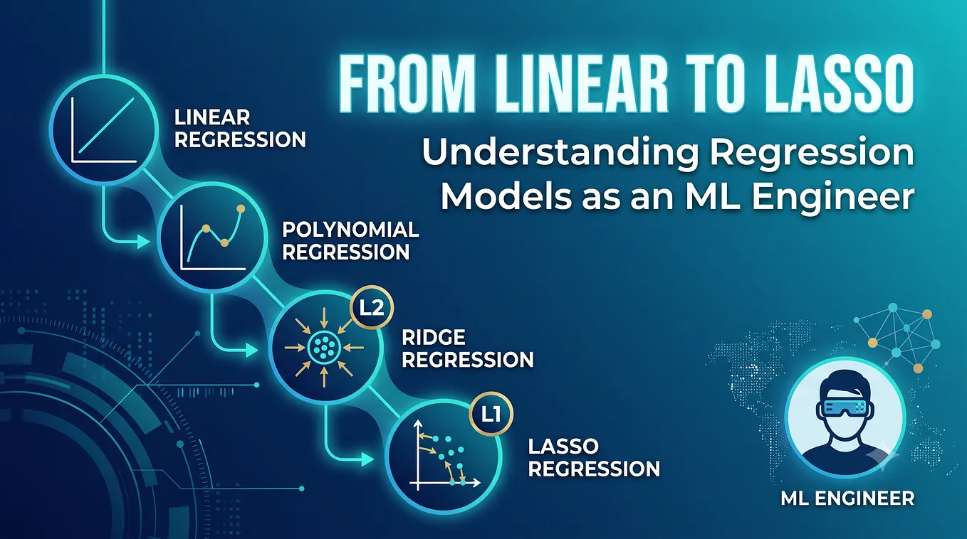
Polynomial Regression: A Complete Beginner-Friendly Guide with Python Implementation
Transforming Linear Regression into Powerful Curved Predictions

Introduction
Machine Learning models are widely used to predict continuous values such as house prices, stock prices, temperature, sales revenue, and much more. One of the simplest regression techniques is Linear Regression, where the relationship between input and output is represented using a straight line.
However, not all real-world data follows a straight-line relationship. Sometimes the relationship between variables is curved or nonlinear. In such cases, Polynomial Regression becomes a powerful solution.
In this guide, we will explore:
- What Polynomial Regression is
- Why it is needed
- Difference between Linear and Polynomial Regression
- Mathematical equations
- Working process
- Advantages and disadvantages
- Overfitting problem
- Python implementation
- Evaluation metrics
- Real-world applications
What is Polynomial Regression?
Polynomial Regression is a supervised machine learning algorithm used to model nonlinear relationships between input (X) and output (Y).
Instead of fitting a straight line, it fits a curve.
Even though it models nonlinear data, it is still considered a type of linear regression because it is linear in terms of coefficients.
Why Do We Need Polynomial Regression?
Linear Regression works well only when the relationship is linear.
Works well for:
- House price increasing with area
- Salary increasing with experience
Fails for:
- Population growth trends
- Stock market fluctuations
- Temperature changes over time
- Sales seasonal patterns
Polynomial Regression helps capture these curved patterns by adding higher-degree terms.
Linear Regression vs Polynomial Regression
Linear Regression
- Relationship: Linear
- Shape: Straight line
- Flexibility: Low
- Complexity: Simple
- Overfitting risk: Low
Polynomial Regression
- Relationship: Nonlinear
- Shape: Curved line
- Flexibility: High
- Complexity: Higher
- Overfitting risk: Higher
Mathematical Equation
Linear Regression
y = β₀ + β₁x
- y = predicted output
- x = input feature
- β₀ = intercept
- β₁ = slope
Polynomial Regression (Degree 2)
y = β₀ + β₁x + β₂x²
Polynomial Regression (Degree 3)
y = β₀ + β₁x + β₂x² + β₃x³
General Form
y = β₀ + β₁x + β₂x² + … + βₙxⁿ
Higher degree → more flexible curve
How Polynomial Regression Works
Polynomial Regression works in 3 steps:
- Take original input features
- Transform them into polynomial features
- Apply Linear Regression on transformed data
Example Transformation
If:
- X = [2]
- Degree = 3
Then transformed features become:
- [1, x, x², x³] → [1, 2, 4, 8]
Understanding Polynomial Features
- Degree 1 → (x)
- Degree 2 → (x, x²)
- Degree 3 → (x, x², x³)
- Degree 4 → (x, x², x³, x⁴)
Higher degree → more complex model

Advantages of Polynomial Regression
- Handles nonlinear data effectively
- Provides better accuracy for curved relationships
- Flexible (degree can be adjusted)
- Easy to implement using Scikit-learn
Disadvantages of Polynomial Regression
- High risk of overfitting (especially high degree)
- Computationally expensive for large datasets
- Sensitive to outliers
- Poor performance in extrapolation (outside data range)
Overfitting in Polynomial Regression
- Low degree → Underfitting
- Medium degree → Good fit
- High degree → Overfitting
Example:
- Degree 1 → too simple
- Degree 2–3 → balanced
- Degree 10 → overly complex curve
Bias–Variance Tradeoff
- Low degree → High bias, low variance
- Medium degree → Balanced
- High degree → Low bias, high variance
Goal: choose optimal degree
Evaluation Metrics
MAE (Mean Absolute Error)
Average absolute error between actual and predicted values.
Get Gilnapradeep’s stories in your inbox
Join Medium for free to get updates from this writer.
MAE = (1/n) Σ |yᵢ — ŷᵢ|
MSE (Mean Squared Error)
Penalizes larger errors more heavily.
MSE = (1/n) Σ (yᵢ — ŷᵢ)²
RMSE (Root Mean Squared Error)
Error in original units.
RMSE = √MSE
R² Score
Measures goodness of fit:
- Closer to 1 → better model
- Closer to 0 → poor model
R² = 1 − (SSres / SStot)
Python Implementation of Polynomial Regression
Step 1: Import Libraries
import numpy as np
import pandas as pd
import matplotlib.pyplot as plt
from sklearn.model_selection import train_test_split
from sklearn.preprocessing import PolynomialFeatures
from sklearn.linear_model import LinearRegression
from sklearn.metrics import mean_absolute_error, mean_squared_error, r2_scoreStep 2: Create Dataset
X = np.array([1,2,3,4,5,6,7,8,9,10]).reshape(-1,1)
y = np.array([1,4,9,16,25,36,49,64,81,100])
Step 3: Split Data
X_train, X_test, y_train, y_test = train_test_split(
    X, y, test_size=0.2, random_state=42
)
Step 4: Polynomial Transformation
poly = PolynomialFeatures(degree=2)X_train_poly = poly.fit_transform(X_train)
X_test_poly = poly.transform(X_test)Step 5: Train Model
model = LinearRegression()
model.fit(X_train_poly, y_train)
Step 6: Predictions
y_pred = model.predict(X_test_poly)Step 7: Evaluation
mae = mean_absolute_error(y_test, y_pred)
mse = mean_squared_error(y_test, y_pred)
rmse = np.sqrt(mse)
r2 = r2_score(y_test, y_pred)
print("MAE:", mae)
print("MSE:", mse)
print("RMSE:", rmse)
print("R2 Score:", r2)Step 8: Visualization
plt.scatter(X, y)X_grid = np.linspace(min(X), max(X), 100).reshape(-1,1)
X_grid_poly = poly.transform(X_grid)plt.plot(X_grid, model.predict(X_grid_poly))
plt.title("Polynomial Regression")
plt.xlabel("X")
plt.ylabel("Y")
plt.show()
Choosing the Best Degree
Instead of a table, here are the approaches:
- Cross-validation
- Grid Search
- Validation score comparison
- Error analysis
Grid Search Example
from sklearn.model_selection import GridSearchCV
from sklearn.pipeline import Pipeline
pipeline = Pipeline([
('poly', PolynomialFeatures()),
('model', LinearRegression())
])param_grid = {
'poly__degree': [1,2,3,4,5]
}grid_search = GridSearchCV(pipeline, param_grid, cv=5, scoring='r2')
grid_search.fit(X, y)print(grid_search.best_params_)
Real-World Applications
- Finance: stock price prediction, revenue forecasting
- Healthcare: disease progression modeling
- Weather: temperature trends
- Engineering: stress–strain curves
- Business: sales forecasting
Polynomial Regression with Multiple Features
For multiple inputs:
- X₁, X₂
Polynomial expansion includes:
- X₁², X₂²
- X₁X₂ (interaction term)
This helps capture feature relationships.
When to Use Polynomial Regression
Use when:
- Data is nonlinear
- Linear regression underfits
- Dataset is moderate in size
Avoid when:
- Dataset is very large
- Overfitting becomes severe
- Relationship is extremely complex
Conclusion
Polynomial Regression extends Linear Regression to handle nonlinear patterns by introducing polynomial features. It is powerful but must be carefully tuned to avoid overfitting.
It is widely used in prediction tasks where data naturally forms curves.
Final Takeaway
Polynomial Regression helps you understand:
- Nonlinear relationships
- Feature transformation
- Overfitting control
- Bias–variance tradeoff
- Model evaluation techniques
It is a strong foundation for advanced machine learning models.
If you understood polynomial regression, you now understand one of the most important foundations of nonlinear machine learning.
What ML topic should I explain next?