Your ML Model Made a Call. Can You Defend It?

You trained a model. 99% accuracy. Validation looks clean, AUC is solid, your team is happy. You ship it. Three weeks later, it flags a high-profile account for spam. The person complains. Your manager walks over and asks
“Why did the model make this call?”
And you realize you don’t actually have a good answer. You know the model is good. You know it works. But you cannot explain a single specific prediction. Not to your manager, not to the user, not to yourself.
A model can be statistically successful and operationally hard to defend.
Lets say that you’re an ML engineer at X (formerly Twitter).
Your job? Flag accounts that are spammy, harmful, or promoting genuinely negative content. You’ve trained a model, it’s performing well, and in a recent run it flagged 500+ accounts across a sample.
Notifications go out. Accounts get suspended.

Now your team lead walks in and asks “What exactly is the model picking up on? What features are driving these flags?”
That’s a fair question, and honestly, a pretty easy one to answer. You just pull up your feature importance scores.
If you’re using a tree-based model like XGBoost or Random Forest, this is built in, so we can use feature importance to understand the contribution of features for the entire data.
Feature importance tells us how decisions were taken for an entire sample
Feature importance is great for this. It tells you the global picture
how the model behaves overall across all 500+ predictions.
But then something else happens. One of those 500 flagged accounts belongs to a well-known influencer. Millions of followers. Verified. And they are not happy. They’ve raised a formal complaint. Their legal team is involved. And now someone in your company needs to explain, not just “the model flagged you,” but why.
What specific factors led to this specific account getting suspended?
This is where feature importance breaks down completely. Feature importance tells you which features matter on average, across the whole dataset. It does not tell you what happened for account #247 out of your 500.
The influencer doesn’t care about averages. They want to know what about their account triggered this. That’s a completely different question and that’s exactly what SHAP Values are built to answer.
SHAP Values
To understand the contribution of each feature for a single prediction we use SHAP Values
- so in our given example we will just plot the shap values for the particular prediction and can get a graph like this

For the influencer’s account, we generated the following SHAP explanation.
- Each bar represents a feature that influenced the model’s decision.
- Features shown in red pushed the prediction towards the “spam/harmful account” class, while features shown in blue pushed it away from that class.
- The length of each bar indicates the magnitude of that feature’s contribution.
In this example, we can observe that:
- A high number of reports from other users strongly pushed the prediction towards the spam category.
- An unusually high posting frequency also increased the probability of the account being flagged.
- Recent account verification status reduced the spam probability and acted as a counter-argument against termination.
- A long account age also contributed positively towards legitimacy.
What makes SHAP powerful is that it doesn’t simply tell us which features are important overall.
Instead, SHAP shows how individual features contributed to the model’s prediction relative to the model’s baseline.
Feature Importance vs SHAP Values
Feature Importance answers:
Which features matter the most across the entire dataset?
SHAP Values answer:
Why did the model make this decision for this specific prediction?
As machine learning systems become increasingly involved in moderation, lending, healthcare, hiring, and recommendation systems, being able to justify individual predictions is often just as important as achieving high accuracy.
SHAP Values provides Interoperability to these black boxes (ML Models) even black-box ones like gradient boosting or neural networks interpretable at the level of a single prediction.
A model that is 99% accurate but cannot explain its decisions may be difficult to trust in production.
Let’s have a hands on practice around SHAP values and utilize them to understand the contribution of each feature for single prediction
we are going to use a Loan Approval Dataset from kaggle
Link to dataset- Loan-approval-prediction-dataset
Link to Google Colab notebook — HandsOnNotebook
0. The Dataset
For this hands-on example, we’ll use the Loan Approval Prediction Dataset published on Kaggle by Archit Sharma.
The dataset contains 4,269 loan applications across 13 columns. It includes applicant information such as education, employment status, annual income, number of dependents, requested loan amount and term, CIBIL score, and different categories of asset value.
Our target variable is loan_status, which contains two outcomes: Approved and Rejected.
The dataset includes the following fields:
no_of_dependents— number of dependentseducation— Graduate / Not Graduateself_employed— Yes / Noincome_annum— annual incomeloan_amount— requested loan amountloan_term— loan termcibil_score— CIBIL credit scoreresidential_assets_value— residential asset valuecommercial_assets_value— commercial asset valueluxury_assets_value— luxury asset valuebank_asset_value— bank asset value
We’ll drop loan_id because it is simply an identifier and does not represent a predictive feature.
Dataset source: Archit Sharma, Loan Approval Prediction Dataset, Kaggle.
1: Import Libraries and Load Dataset
import pandas as pd
import numpy as np
import xgboost as xgb
import shap
from sklearn.model_selection import train_test_split
from sklearn.preprocessing import LabelEncoder
df = pd.read_csv("loan_approval_dataset.csv")
df.head()
2: Encode Categorical Features
Machine Learning models cannot directly understand text values. so we are encoding them using LabelEncoder Class of scikit Learn
le_education = LabelEncoder()
le_self_employed = LabelEncoder()
le_target = LabelEncoder()
df["education"] = le_education.fit_transform(df["education"])
df["self_employed"] = le_self_employed.fit_transform(df["self_employed"])
df["loan_status"] = le_target.fit_transform(df["loan_status"])
X = df.drop(["loan_id", "loan_status"], axis=1)
y = df["loan_status"]
3: Train The ML Model
X_train, X_test, y_train, y_test = train_test_split(
    X,
    y,
    test_size=0.2,
    random_state=42
)
Tree-based models work extremely well with SHAP.
Get Moksh’s stories in your inbox
Join Medium for free to get updates from this writer.
Train an XGBoost Model
model = xgb.XGBClassifier(
    max_depth=4,
    n_estimators=100,
    learning_rate=0.1,
    eval_metric="logloss"
)
model.fit(X_train, y_train)
4 : Generate SHAP Values
we create an explainer object and pass all values of test in explainer object
explainer = shap.Explainer(model)
shap_values = explainer(X_test)
At this point, SHAP has calculated how much each feature contributes to every prediction.
5 : Global Feature Importance
Let’s first understand which features matter most across the entire dataset.
shap.plots.bar(shap_values)
This gives us a dataset-level view.
For example, we might observe that:
- CIBIL Score has the largest influence
- Income plays a major role
- Asset values affect approval decisions
This is similar to traditional feature importance, Individual Prediction Explanation
Now let’s inspect a single applicant.
shap.plots.waterfall(shap_values[0])
This is where SHAP becomes truly useful.
Instead of explaining the model globally, it explains a single decision.
The waterfall chart tells us:
- Which features pushed the prediction toward approval
- Which features pushed it toward rejection
- The magnitude of each contribution
For example:
- High CIBIL score pushes the model output toward approval.
- High annual income may further support approval
- Large loan amount may decrease approval probability
Together these factors produce the final prediction.
6 : Understanding Feature Behavior Across All Applicants
shap.plots.beeswarm(shap_values)
The beeswarm plot combines the local SHAP explanations for the predictions in our test set into a single visualization.
It answers questions such as:
- Does a higher CIBIL score generally increase approval chances?
- Does income consistently help?
- Which features have the largest variation in impact?
This plot is often the most informative SHAP visualization in real-world projects.
Results:
Now that we’ve looked at the global feature importance, individual prediction, and feature behavior across the test set, we can see what the model is actually learning.
Globally, cibil_score is the dominant feature, with a mean absolute SHAP value of 8.12, followed by loan_term (3.35), income_annum (2.17), and loan_amount (1.77).
For the individual applicant, the waterfall plot tells a different story. The applicant’s cibil_score of 423 contributed +6.49, while loan_term contributed +6.12. Both pushed the model strongly toward the Rejected class. Meanwhile, loan_amount contributed −2.94, partially offsetting those contributions.
The beeswarm plot helps us generalize beyond this one applicant. For cibil_score, lower values tend to produce positive SHAP values and push predictions toward rejection, while higher values generally push them toward approval.
This is the key difference between a global feature ranking and a local explanation: one tells us what matters to the model overall, while the other shows how those features contributed to a specific prediction.
Conclusion
Looking at our three SHAP plots, we can see the difference clearly.
The global plot tells us what the model relies on most — in our case, cibil_score stands out as the dominant feature, followed by loan_term, income_annum, and loan_amount.
The waterfall plot takes us one level deeper. Instead of looking at the model as a whole, we can inspect one applicant’s prediction and see how individual features pushed the model output up or down.
And the beeswarm plot brings us back to the bigger picture, showing how those feature contributions behave across the entire test set.
That’s the real value of SHAP. It doesn’t just give us another feature-importance score. It gives us a way to move from:
“What does my model care about?”
to:
“How did those features contribute to this particular prediction?”
A model’s accuracy tells us whether it performs. SHAP helps us understand how it behaves.
And when we’re putting ML models into systems where individual predictions matter, understanding that difference can be just as important as the prediction itself.
What SHAP doesn’t Tell you?
SHAP explains how the model uses its input features. It does not prove that those features caused the outcome in the real world.
It also doesn’t tell us whether the model is fair, whether the data is unbiased, or whether the model’s decision is correct.
An explanation of a model’s decision is not the same thing as a justification of that decision
Now, SHAP works great when you already have labels, spam or not spam, approved or rejected. But what happens when you don’t?
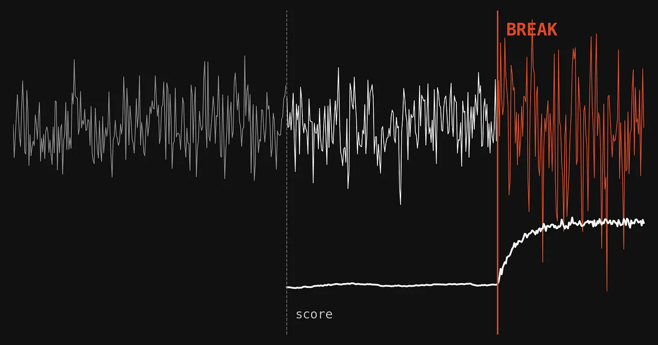
What if you’re trying to catch the accounts that don’t look like anything in your training data at all? No history of being flagged, no labeled examples to learn from, just… weird.
That’s a completely different problem, anomaly detection, and it’s where Isolation Forest comes in. We’ll get into that next.
Tools, Data & Resources
This article was built using the following open-source tools and public resources:
- SHAP — SHapley Additive exPlanations, an open-source framework for interpreting machine-learning model outputs. The project is supported by the German Center for Open Source AI (GC.OS). GitHub
- scikit-learn — Used for preprocessing and the train/test split, including
LabelEncoderandtrain_test_split. Scikit-learn - XGBoost — Used to train the gradient-boosted tree classifier that we explain with SHAP. SHAP provides optimized support for explaining tree-ensemble models such as XGBoost. GitHub
- Loan Approval Prediction Dataset — Dataset by Archit Sharma, sourced from Kaggle. Kaggle
- Google Colab Notebook — Full implementation and experiments accompanying this article.
Direct links
SHAP: GitHub Repository
SHAP Documentation: SHAP Documentation
scikit-learn: scikit-learn Documentation
XGBoost: XGBoost Documentation
Dataset: Loan Approval Prediction Dataset on Kaggle
Notebook: Google Colab Notebook
About the Writer
Heyyy folks , This side Moksh. I am an undergrad who is interested in everything around Data and AI, will be writing more such handson Blogs around niche topics around ML or AI so do subscribe
Subscribe now