How Easy Is It to Start Serving LLMs?
How we stood up Qwen3 on a single A10 or A100 from a plain Ubuntu box, benchmarked it, and opened up FlashInfer to see why it works. All code is open-sourced.
By the Geodesic OSS team
Inference providers like Fireworks, Baseten, and Together have built big businesses on a simple promise: click a few buttons and an open-source model such as Qwen, Kimi, or MiniMax is serving traffic behind an API. For a startup running at scale, that convenience can add up to millions of dollars a year.
So we asked a simple question: how hard is it, really, to serve an open-source LLM yourself?
The answer surprised us. Starting from a plain Ubuntu GPU machine, setup takes about three minutes, and what you get is not a toy. It is a real serving system with a prefix KV cache, chunked prefill, continuous batching, paged GPU memory management, JIT-compiled attention kernels, and GPU load balancing, behind an OpenAI-compatible API with streaming and tool calls.
In this post, we walk through the whole thing step by step: setup, validation, a stress test with TTFT and ITL numbers, and a look inside the kernels. Everything runs from nine scripts we have open-sourced in geodesic/aees/serving.
TL;DR
- Setup: two commands take a fresh Ubuntu 24.04 GPU host to a running Qwen3–4B server.
- Latency: on one A100, a single user gets the first token in about 220 ms and then a new token every ~9 ms. At 64 concurrent requests, inter-token latency stays under 35 ms at p99.
- What matters most: the prefix cache is the biggest lever for agent traffic (turning it off cuts throughput by 59%), and FlashInfer beats Triton by 17% in throughput.
- Inside FlashInfer: scattered KV pages read at 99–101% of the speed of contiguous ones, each new attention variant compiles once in 7–15 s and then loads in under 1 ms, and the scheduler costs ~3 µs per layer.
The stack: open-source layers, end to end
None of this is our invention. We stand on three layers of open-source work, and our scripts are the glue that installs, runs, and measures them.

- SGLang, the serving runtime, decides what runs: it batches requests continuously, caches shared prompt prefixes in a radix tree (RadixAttention), splits long prompts into chunks so they don’t stall everyone else, and exposes an OpenAI-compatible API.
- FlashInfer, the kernel library, decides how attention runs on the GPU: it reads a paged KV cache through block-sparse indices, compiles exactly the attention variant a model needs, and balances work across the GPU’s streaming multiprocessors (SMs).
- PyTorch and CUDA sit underneath, on one NVIDIA A10 (24 GB) or A100 (40 GB).
Four phases, nine scripts
Phases 1–2: stand it up. setup_host.sh takes a fresh Ubuntu 24.04 machine to a working stack. It installs the NVIDIA driver (if needed) and the CUDA 13 toolkit, creates a Python environment, installs SGLang, and installs FlashInfer's prebuilt kernels pinned to exactly the FlashInfer version SGLang pulled in (a mismatch here is the most common way this goes wrong). It finishes by checking a FlashInfer attention kernel against a plain PyTorch reference. serve.sh start then launches Qwen3-4B with FlashInfer attention, the prefix cache and Prometheus metrics, inside a tmux session, and waits until the API answers.
Phase 3: validate and stress-test. smoke_test.py runs from your laptop through an SSH tunnel. It checks a plain chat reply, a tool call and a prefix-cache hit, then drops you into an interactive chat. run_bench.py is the stress test. It restarts the server once per configuration (baseline, prefix cache off, FP8 KV cache, page size 16, Triton instead of FlashInfer) and drives SGLang's own load generator through concurrency sweeps, a Poisson QPS sweep, a long run for p99.9 tails and a burst of simultaneous requests. make_dashboard.py turns the per-request results into one interactive HTML dashboard.
Phase 4: look inside FlashInfer. run_phase4.sh runs three microbenchmarks at Qwen3-4B's exact attention shapes (32 query heads, 8 KV heads, head dimension 128) and one live capture, then builds a report:
- Sparse KV memory:
fi_bench.py sparsetests how page size and page scattering affect memory bandwidth. - JIT compilation:
fi_bench.py jittimes first-use compilation of ten attention variants, in a clean environment built byfi_jit_setup.sh. - Load balancing:
fi_bench.py balancetests how the scheduler copes with skewed request lengths. - Live capture:
fi_trace.pyhooks the running server and records the real KV index arrays while traffic flows.
# On the GPU host, from geodesic/aees/serving/
bash setup_host.sh        # Phases 1–2: driver, CUDA, SGLang, FlashInfer, model weights
./serve.sh start          # Qwen3-4B on 127.0.0.1:30000
python run_bench.py       # Phase 3: stress test → results/<run>/dashboard.html
./run_phase4.sh           # Phase 4: FlashInfer deep dive → results/fi/fi_report.html
About three minutes. On a cloud GPU image with the NVIDIA driver preinstalled (as on Lambda), hands-on time is roughly three minutes. On bare metal, the driver install adds one reboot.
Phase 3 results: TTFT, ITL and what matters most
We measured two latencies, because users feel them differently:
- TTFT (time to first token) is the pause before a response starts streaming. It covers queueing plus prefill, the work of processing the whole prompt.
- ITL (inter-token latency) is the gap between tokens once streaming has started. It sets how fast text appears.
All Phase 3 numbers are from one A100–40GB running Qwen3–4B in BF16 with SGLang 0.5.21 and FlashInfer 0.6.18. The main workload is agent-like: 16 different 4,000-token system prompts (think prompt templates plus tool schemas), each followed by a short question and a 256-token answer.

Key latency results
- Single user: TTFT 217 ms median and 221 ms p99; ITL 8.5 ms median, roughly 118 tokens per second while streaming.
- 16 concurrent requests: median TTFT stays at 281 ms, but p99 rises to 2.0 s. ITL stays at 13.8 ms median and 14.8 ms p99. Total throughput is 935 output tokens/s.
- 64 concurrent requests: median TTFT 1.05 s, p99 3.8 s. ITL 30.9 ms median and 34.5 ms p99. Throughput peaks at 1,576 tokens/s.
- Tails, from a 400-request run at 64 concurrent: TTFT p50 / p99 / p99.9 = 989 / 4,030 / 4,031 ms. ITL p50 / p99 / p99.9 = 31 / 39 / 550 ms. The rare 550 ms gaps are moments when a stream pauses while new prompts are prefilled.
- Reliability: 0 failed requests out of 2,082, including a burst of 304 requests sent at the same instant (TTFT p99 6.0 s under that burst).
The headline is that streaming stays fast under load, and time to first token is the constraint. Against a strict 500 ms p99 TTFT target, this run met the target only at a single concurrent request. One caveat makes that conservative: the benchmark empties the prefix cache before every test and launches all requests at once, so the first wave of each test misses the cache together. In steady agent traffic, shared prompts stay cached and first-token latency is lower.

What each setting does to performance
- Turn off the prefix cache: throughput −59%, TTFT p99 +424% (to 20 s). Without it, every request recomputes its 4,000-token system prompt. For agents, which resend the same instructions and tool schemas on every step, this is the most important feature in the stack.
- Replace FlashInfer with Triton attention: throughput −17%, TTFT p99 +21%, ITL p99 +27%. Same GPU, same model; the difference is the attention kernels and scheduler.
- FP8 KV cache: throughput −5%, ITL p99 +17%. On the A100, FP8 is a capacity tool, not a speed tool. It roughly doubles how many tokens fit in the KV cache, but the A100 has no FP8 math units, so every value is converted back to 16-bit as it’s read. It pays off only when memory, not compute, is the limit: long contexts or many concurrent sessions.
- KV page size 16 instead of 1: no measurable change (±1%). Phase 4 explains why.
Phase 4: inside FlashInfer
Phase 3 showed that FlashInfer helps. Phase 4 asks how, by testing its three core ideas one at a time on an NVIDIA A10 (72 SMs, 600 GB/s memory bandwidth).
1. Block-sparse KV memory: scattered pages cost nothing
A serving engine can’t give each request one long contiguous slab of memory for its KV cache. Requests grow token by token, finish at different times, and share prompt prefixes. So the KV cache is a pool of fixed-size pages, and each request is a list of page numbers that can sit anywhere in the pool.
Get Will Youzhi Zou’s stories in your inbox
Join Medium for free to get updates from this writer.
FlashInfer treats that page table as a sparse matrix: one row per request, one column per physical page. Three small arrays describe it, and they are all the attention kernel needs:
# Illustration: a batch's KV pages, described in CSR form
kv_indptr, kv_indices = [0], []
for req in batch:
    kv_indices += req.page_ids         # pages, anywhere in pool
    kv_indptr.append(len(kv_indices))  # end of this request's row
# Request i reads:
#   pool[kv_indices[kv_indptr[i] : kv_indptr[i + 1]]]
# Requests sharing a prompt just list the same page ids.

Key results
- Scattered pages read at 99–101% of the speed of contiguous pages, for every page size (1, 4, 16, 64) and every batch shape tested (64 × 4K, 16 × 16K and 256 × 1K tokens).
- Decode reaches 490–501 GB/s, over 80% of the A10’s 600 GB/s peak. Attention at decode time is a memory-bandwidth problem, and FlashInfer keeps the memory system busy.
- Why page size doesn’t matter: even a single-token page is a 2 KB contiguous read per layer (8 KV heads × 128 dims × 2 bytes), already large enough for efficient memory transfers. Larger pages mainly shrink the bookkeeping, from 262K index entries per batch at page size 1 to 16K at page size 16.
- FP8 KV halves the bytes but is only about 3–9% faster at the kernel level on the A10, because converting each value back to 16-bit eats most of the saving. This matches the Phase 3 finding on the A100.
- Live capture from the running server: agent batches showed each KV page referenced by up to ~3.5 requests on average, which is the prefix cache at work. As traffic churned, the pool fragmented from runs of thousands of contiguous pages down to runs of just a few. Thanks to the result above, that fragmentation costs nothing.
2. JIT compilation: one template, a kernel per variant
Attention comes in many variants: different data types, head sizes, position encodings, logit soft-capping, sliding windows. Shipping a precompiled kernel for every combination isn’t practical. FlashInfer instead keeps one CUDA template per kernel family and compiles the exact variant a model needs the first time it’s used:
# Illustration: FlashInfer's just-in-time kernel path
key = (dtype_q, dtype_kv, head_dim, mask, pos_enc,
       soft_cap, gpu_arch)
if key not in jit_cache:
    src = render_template("batch_decode.cu", key)
    jit_cache[key] = nvcc_compile(src)   # slow, once
kernel = jit_cache[key]                  # fast, every call

Key results
- Each new variant costs 7.0–14.9 s on first use and 0.2–0.6 ms afterwards, a speedup of more than 10,000×.
- Variants differ only in template parameters. Diffing the generated source for the base decode kernel and the soft-cap variant shows exactly two changed lines:
USE_LOGITS_SOFT_CAP = false → trueand the matching template argument. - Compiled modules are shared. Decoding on tensor cores reuses the prefill kernel, so the batch-prefill variant that ran next compiled nothing at all.
- What it means in production: install FlashInfer’s prebuilt kernel wheels (
setup_host.shdoes this) and keep the JIT cache on persistent disk, so restarts never pay the compile cost.
3. Load balancing: keep every SM busy
During decoding, every request in a batch needs attention over its entire history, and histories vary wildly. One agent session might have 30,000 tokens of context while its neighbors have 500. If each request is assigned to one SM, the whole step waits for the longest request while the other SMs sit idle.
FlashInfer splits this into plan and run. Once per decode step, plan() runs on the CPU, looks at the current lengths, splits long requests into chunks and packs chunks onto SMs evenly. Every layer then reuses that plan, and a small merge step stitches the chunks of each long request back together:
# Illustration: split-KV planning (simplified)
def plan(kv_lens, num_sms):
    target = sum(kv_lens) / num_sms      # ideal work per SM
    queues = [[] for _ in range(num_sms)]
    longest_first = sorted(enumerate(kv_lens),
                           key=lambda r: -r[1])
    for req, n in longest_first:
        for chunk in split(n, max_len=target):
            lightest = min(queues, key=total_work)
            lightest.append((req, chunk))
    return queues  # to GPU once; reused by all 36 layers

Key results
- Scheduling is nearly free.
plan()costs ~2.5–2.8 µs per layer (once per step, amortized across 36 layers), against ~150–8,000 µs of attention work per layer for batches of 8 to 512 requests. - With few requests, skew costs nothing. At 4 and 16 requests, the decode kernel took the same time whether lengths were uniform, one very long request among short ones, or heavy-tailed. The scheduler fully absorbed the imbalance.
- With many requests, skew starts to show. At 64 and 128 requests, skewed mixes ran roughly 1.2–1.8× slower than uniform ones with the same total tokens. That fits a sensible trade-off: once there are enough requests to fill every SM, splitting buys less and costs a merge step, so the longest request again sets the pace. This FlashInfer version doesn’t expose a switch to disable splitting, so we measured how the balancer handles skew rather than comparing it on and off.
- CUDA-graph friendly. Because the plan lives in a fixed GPU buffer, the per-step kernels can be captured once as CUDA graphs and replayed, which keeps launch overhead low.
Demo: talk to your model from a laptop
The server listens only on 127.0.0.1 on the GPU host, so nothing is exposed to the internet. Your laptop reaches it through an SSH tunnel over port 22, which on Lambda is the only port open by default. One tunnel carries both the model API and the results dashboards.

1. On the GPU host, start the server and print the tunnel command:
cd geodesic/aees/serving
./serve.sh start        # waits until Qwen3-4B answers, then prints a test reply
./serve.sh dashboard    # serves benchmark results on 127.0.0.1:8000
./serve.sh tunnel       # prints the exact SSH command for your laptop
2. On your laptop, open the tunnel and leave it running:
ssh -N -L 30000:127.0.0.1:30000 -L 8000:127.0.0.1:8000 ubuntu@<gpu-host-ip>3. In a second laptop terminal, run the smoke test, then chat:
pip install openai
python smoke_test.py               # 3 checks, then: "Start an interactive chat? [Y/n]"
python smoke_test.py chat --tools  # straight into chat, with a demo weather tool
A session looks like this (the model’s wording will vary). Replies stream token by token, and each turn reports its TTFT and total time:
=== Interactive chat with the model (stdin/stdout) ===
Tools: ON (demo get_weather; try: what is the weather in Paris?)
Commands: /tools (toggle)  /reset  /system <text>  /history  /quit
you> what's the weather in Paris?
bot> (calling a tool)
      (TTFT … ms, total … s)
tool> get_weather({"city": "Paris"}) -> {"city": "Paris", "temperature": 21, "unit": "celsius", "conditions": "sunny (demo data)"}
bot> It's currently 21°C and sunny in Paris.
      (TTFT … ms, total … s)
Because the server speaks the OpenAI API, anything that works with OpenAI works here: the official SDK, agent frameworks, or plain curl. Point it at http://127.0.0.1:30000/v1 and use the model name qwen3-4b:
from openai import OpenAI
client = OpenAI(base_url="http://127.0.0.1:30000/v1", api_key="none")
reply = client.chat.completions.create(
    model="qwen3-4b",
    messages=[{"role": "user", "content": "Explain KV caching in one sentence."}],
)
print(reply.choices[0].message.content)
The Phase 3 dashboard and the Phase 4 report open in your browser at http://127.0.0.1:8000/.
Conclusion: serving is easy now, thanks to open source
Standing up a capable LLM server is no longer a specialist project. On one rented A10 or A100, about three minutes of setup gives you a system with the same core machinery the big providers advertise: prefix caching, chunked prefill, continuous batching, paged memory, tuned attention kernels and GPU load balancing.
That is possible because of layers of open-source work, each solving a hard problem so the next layer doesn’t have to:
- Low-level kernels: FlashInfer’s attention templates and CUDA code.
- Mid-level GPU systems: block-sparse memory management, just-in-time kernel compilation, and load-balanced scheduling.
- High-level serving strategy: SGLang’s prefix (radix) KV cache, chunked prefill and continuous batching.
Our contribution is small by comparison: the scripts that install, run, measure and explain this stack, so anyone can reproduce it and see what each piece is worth.
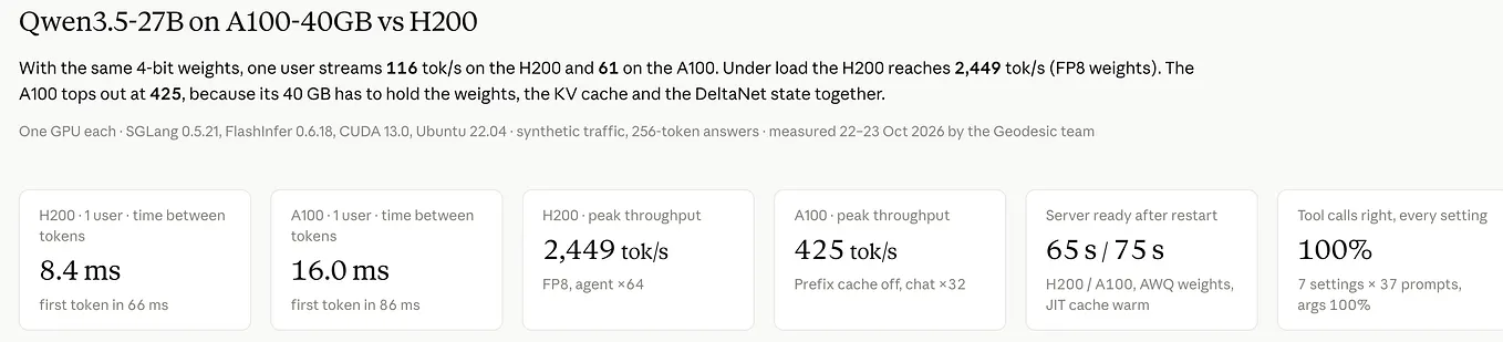
What’s next. We’ll follow up with a 27B-class model, where memory pressure, multi-GPU parallelism and FP8 become the main story. For Geodesic, serving is a means, not the end. Our goal is to advance reinforcement learning and long-horizon agentic tasks, and both run on fast, cheap, controllable inference: thousands of agent steps, long shared contexts and many parallel rollouts. We’ll keep building in that direction, in the open.
Try it: the code is at github.com/anglenexus/geodesic, aees/serving, along with the full Phase 3 dashboard and Phase 4 report as PDFs. Issues and pull requests are welcome.
Setup: Qwen3–4B (BF16) on SGLang 0.5.21 and FlashInfer 0.6.18 with PyTorch 2.13 and CUDA 13.0. Phase 3 on an NVIDIA A100-SXM4–40GB; Phase 4 on an NVIDIA A10. Phase 3 numbers come from a single quick benchmark pass, so differences under about 5% are within noise. A few Phase 4 values (plan() cost, kernel time, FP8 and skew ratios) are read from charts and marked as approximate.