
An analog computer in the browser: a rack of instruments for dynamical systems and audio signals. The core is Go compiled to WebAssembly; the same program runs on the host as a terminal panel, a native rack and a renderer. An homage to the analog computers at glensstuff.com.
Live demo · TinyGo build · Model pages · Manual

- 79 models. Flows (Lorenz, Rössler, Chua, Sprott A–S, 4-D hyper-Rössler, …), maps (Hénon, Ikeda, Clifford, de Jong, Gumowski–Mira, Tinkerbell, Chirikov), parametric figures, an integer-sequence turtle with rigid-body physics, geometry and STL solids, terminals and a desktop drawn into the scene, delay embeddings of live audio, audio analyzers, and a ripple tank.
- A rack control surface. Programmable encoder banks, selector knobs with LED rings, seven-segment and dot-matrix displays, a pin-matrix Mixer and Mod matrix, four oscilloscopes and four signal generators.
- Audio in and out. Microphone, built-in generators (0.1 Hz – 28 kHz), or
this machine's audio streamed by the server (
--audio). Any parameter can be driven by the signal; Model Out plays the model's own equations. - Measurement. Largest Lyapunov exponent, bifurcation, recurrence; THD+N, RTA, transfer function, LUFS, wow & flutter, waterfall.
- Custom systems typed as derivatives or maps; permalinks and presets; WebM/GIF recording.
- Contents
- Run
- Features
- Models
- Controls and measurement
- Remote access
- The rack
- Physical dimensions
- Solid models (STL)
- Recording
- Gallery
- Audio
- FVF — Harmonic Wobbulator
- Testing & tooling
- Build
- Related / prior art
- Dependency Graph
- Lines of Code
The WebAssembly is embedded in the binary; there is no build step.
go install github.com/0magnet/chaosrack@master
chaosrack serve            # serve the rack at http://127.0.0.1:8080/
chaosrack serve --audio    # also stream this machine's audio to the page
Or without installing: go run github.com/0magnet/chaosrack@master serve --audio.
Open 127.0.0.1:8080/ (Go build) or 127.0.0.1:8080/tinygo/ (TinyGo build).
--audio records the default PulseAudio/PipeWire monitor — whatever this
machine is playing — and the page connects to it by itself. Without it the page
uses the microphone or the built-in generators.
The page at chaosrack.magnetosphere.net can take its audio and rack link from a server on your own machine, so you don't need to open a page that server serves itself:
- Run
chaosrack serve --audio --pair. It prints a link to the live demo:https://chaosrack.magnetosphere.net/#…&pair=…&wt=127.0.0.1:8080. - Open that link once, in the browser you'll use.
- Allow the browser's prompt to let the site reach "other apps and services on this device" (Local Network Access). Until it's allowed, the page waits and its console says why.
That browser is now paired: plain visits to the demo reconnect by themselves,
even after the server restarts. Each run prints a new link, which only a
browser that hasn't paired yet needs. The paired browsers are listed in
~/.config/chaosrack/paired-tabs; delete a line to unpair one.
For a browser on another machine, run chaosrack serve --bind 0.0.0.0 --audio
and open the link it prints there. WebTransport doesn't go through a proxy, so
if that browser uses one, add this machine's address to its bypass list.
Details, and the threat model: docs/remote-access.md.
serve flag |
|
|---|---|
--audio |
stream system audio to the page (--audio-source default for the input instead of the monitor) |
-p, --port |
port, default 8080 |
-b, --bind |
address, default 127.0.0.1; 0.0.0.0 serves the LAN by pairing |
--pair |
on loopback: pair the public page in a browser on this machine, so it gets this server's audio (how) |
--shell, --fs |
a real shell and filesystem in the page's desk — see Remote access |
--wobbulate |
route system audio through the FVF wobbulator |
Other commands, which also run in the page's own terminal:
| command | |
|---|---|
chaosrack |
the rack's panel in this terminal |
chaosrack ctl [id[=value] …] |
list, read or set any control of a running page |
chaosrack mem [--watch 10s] |
what a running page's memory goes on: the wasm heap and module, the JavaScript heap, elements, canvases, and the JS values Go holds; from a host (--attach), also the tab's footprint as Brave counts it and what it is made of. --watch prints rates over time; a page opened with ?diag also counts calls by name |
chaosrack render --model lorenz -o lorenz.png |
draw a model to PNG, SVG or GIF without a browser, or a video with sound (--audio-file song.flac -o song.mp4) |
chaosrack models · chaosrack manual · chaosrack rack |
list models · read the manual · draw the bays as text |
chaosrack stlgen |
write the rack and the models as STL |
The page also runs with no server at all: see SERVERLESS.md.
- Flows are integrated in the page every frame; every built-in flow's defaults are tested in CI for a positive largest Lyapunov exponent under the app's own integrator.
- Maps have no dt and are drawn as points. Hénon's determinant (−b) and Chirikov's (1) are asserted in tests. The standard map is drawn as an ensemble of orbits; its invariant curves break up as K passes 0.9716.
- Custom equations: type
dx/dt,dy/dt,dz/dt(optional 4th dimension); every named parameter gets a knob. iterate reads the same expressions as a map. - Turtle Path walks an integer sequence mod m (period: the Pisano period) in 2-D or 3-D, classifies the result (closed, drifting, helical), and can be given mass and dropped into a box. Built on 0magnet/pisano.
- Analysis: largest Lyapunov exponent of whatever is on screen, per unit time for flows and per iterate for maps; a bifurcation explorer; a recurrence plot.
- Delay embeddings of live audio: Takens (τ measured by average mutual information, dimension by false nearest neighbors), stereo and polar.
- Trails: scan (the whole curve re-integrated each frame) or Ring (only the head advances); Persist accumulates frames; Points breaks the line into N points.
- Color: the gradient follows x, y, z, trail position or the audio spectrum, through the two-color, three-color, hue or six colormaps shared with the spectrogram (heat, blue, gray, turbo, viridis, magma). CRT phosphor presets with afterglow.
- Generators: four, sine to noise plus test signals (pink noise, log sweep, polarity pulse, …), 0.107 Hz – 28 160 Hz on an octave-a-turn encoder. Below ~20 Hz they are modulators.
- Model Out runs the model's equations at audio rate; its x, y, z are Mixer columns, playable and measurable.
- Mixer: every source (capture, generators, Model Out, keys, drums, tone matrix) is a column of one pin matrix; rows are the speakers, the rack's signal (read by the scopes, meters and models) and two modulation sends.
- Mod matrix: any model or view parameter driven by the rack's signal, a send or the model's own position, with depth, EQ band weighting and a shape (push, swing, flip, or wave — the signal itself).
- Terminals and desk: websh (Bash compiled to wasm) on a quad in the scene; a desk window manager over or inside the scene, with four reproduced 3-D desktops. See docs/desk.md.
- State: permalinks carry the full state; named presets use the same serialization; the rack layout persists.
- Recording: WebM via
MediaRecorderor GIF encoded in Go, full canvas or a region. - Audio transport: float32 samples over WebSocket, or unreliable WebTransport datagrams for lossy links, with automatic fallback.
Also published as one page per model at
chaosrack.magnetosphere.net/models/,
each with its equations, figure and a link that opens it running. Both this
section and those pages are generated from attractor.Catalog(), the
selector's own registry (make site, make site-check).
Every position of the MODEL selector, in knob order; a model in two
categories is listed in both. Per model: its bank as programmed for it,
a still, an animated loop, its description (the Info overlay's text) and
its equations. Images are captured by uitool portraits.
Rossler · Lorenz · Chua · Aizawa · Sprott · Thomas · Halvorsen · Chen · Dadras · Rabinovich-Fabrikant · Burke-Shaw · Lü · Newton-Leipnik · Arneodo · Chen-Lee · Dequan Li · Three-Scroll · Wang-Sun · Lorenz Mod 2 · Simone · Rucklidge · Genesio-Tesi · Shimizu-Morioka · Rikitake Dynamo · Moore-Spiegel · Bouali · Lorenz-84 · Finance · Hindmarsh-Rose · Wei (no equilibrium) · Sprott Jerk · Hyper-Rössler (4D) · Sprott Morph · Sprott A · Sprott B · Sprott C · Sprott D · Sprott E · Sprott F · Sprott G · Sprott H · Sprott I · Sprott J · Sprott K · Sprott L · Sprott M · Sprott N · Sprott O · Sprott P · Sprott Q · Sprott R · Sprott S · Custom equation

| Rossler | animated |
|---|---|
 |
 |
Rössler Attractor — Proposed by Otto Rössler in 1976 as a simpler system that produces chaotic behavior. Unlike the Lorenz system's two-lobed shape, the Rössler attractor has a single folded-band structure with an outward spiral that occasionally makes a large excursion in the z-direction.
dx/dt = −(y + z)
dy/dt = x + ay
dz/dt = b + z(x − c)
#rossler · 3-D flow

| Lorenz | animated |
|---|---|
 |
 |
Lorenz Attractor — Discovered by Edward Lorenz in 1963 while modeling atmospheric convection. The butterfly-shaped trajectory arises from a simplified system of three coupled differential equations. It was one of the first systems shown to exhibit deterministic chaos, where tiny differences in initial conditions lead to vastly different outcomes.
dx/dt = σ(y − x)
dy/dt = x(ρ − z) − y
dz/dt = xy − βz
#lorenz · 3-D flow

| Chua | animated |
|---|---|
 |
 |
Chua's Circuit (Double Scroll Attractor) — Invented by Leon Chua in 1983, this is the first electronic circuit proven to exhibit chaos. The system features a piecewise-linear nonlinearity (the Chua diode) that creates the characteristic double-scroll pattern. It is also the basis for multi-scroll attractor generalizations.
dx/dt = α(y − x − h(x))
dy/dt = x − y + z
dz/dt = −βy
h(x) = m₁x + ½(m₀ − m₁)(|x+1| − |x−1|)
#chua · 3-D flow

| Aizawa | animated |
|---|---|
 |
 |
Aizawa Attractor — A chaotic system that produces a toroidal structure with a tendril extending from the center. The attractor has a visually striking shape that resembles a sphere with a tail, exhibiting both rotational symmetry and chaotic wandering.
dx/dt = (z − b)x − dy
dy/dt = dx + (z − b)y
dz/dt = c + az − z³/3 − (x² + y²)(1 + ez) + fzx³
#aizawa · 3-D flow

| Sprott | animated |
|---|---|
 |
 |
Sprott Attractor — One of many simple chaotic systems cataloged by Julien Clinton Sprott. These systems were discovered through systematic computer searches for chaotic flows with minimal terms, demonstrating that chaos can arise from remarkably simple equations.
dx/dt = y + Axy + xz
dy/dt = 1 − Bx² + yz
dz/dt = x − x² − y²
#sprott · 3-D flow

| Thomas | animated |
|---|---|
 |
 |
Thomas' Cyclically Symmetric Attractor — Introduced by René Thomas, this system has the elegant property of cyclic symmetry: each variable is damped and driven by the sine of the next variable in the cycle. The parameter b controls dissipation; as b decreases the system transitions from stable points through limit cycles to chaos.
dx/dt = −bx + sin(y)
dy/dt = −by + sin(z)
dz/dt = −bz + sin(x)
#thomas · 3-D flow

| Halvorsen | animated |
|---|---|
 |
 |
Halvorsen Attractor — A chaotic system with three-fold rotational symmetry, producing a distinctive pinwheel-like shape. The attractor consists of three intertwined lobes that spiral around each other, creating a visually complex but structurally symmetric trajectory.
dx/dt = −ax − 4y − 4z − y²
dy/dt = −ay − 4z − 4x − z²
dz/dt = −az − 4x − 4y − x²
#halvorsen · 3-D flow

| Chen | animated |
|---|---|
 |
 |
Chen Attractor — Discovered by Guanrong Chen in 1999, this system was found as a dual of the Lorenz system in a specific mathematical sense. It exhibits chaotic behavior with a distinctive two-scroll structure that differs from both the Lorenz and Rössler attractors.
dx/dt = a(y − x)
dy/dt = (c − a)x − xz + cy
dz/dt = xy − bz
#chen · 3-D flow

| Dadras | animated |
|---|---|
 |
 |
Dadras Attractor — A three-dimensional autonomous chaotic system with five parameters, introduced by Sara Dadras and Hamid Reza Momeni. The system exhibits rich dynamical behavior including period-doubling routes to chaos.
dx/dt = y − px + qyz
dy/dt = ry − xz + z
dz/dt = sxy − ez
#dadras · 3-D flow

| Rabinovich-Fabrikant | animated |
|---|---|
 |
 |
Rabinovich-Fabrikant Attractor — Derived by Mikhail Rabinovich and Anatoly Fabrikant from physical equations modeling the stochasticity of three interacting waves. The system is known for its complex topology and extreme sensitivity to parameters, producing intricate folded structures.
dx/dt = y(z − 1 + x²) + γx
dy/dt = x(3z + 1 − x²) + γy
dz/dt = −2z(α + xy)
#rabinovich · 3-D flow

| Burke-Shaw | animated |
|---|---|
 |
 |
Burke-Shaw Attractor — Introduced by Bill Burke and Robert Shaw, this system exhibits chaotic behavior with a distinctive two-winged structure. It arises from the study of nonlinear dynamics and produces complex trajectories confined to a compact region of phase space.
dx/dt = −S(x + y)
dy/dt = −y − Sxz
dz/dt = Sxy + V
#burkeshaw · 3-D flow

| Lü | animated |
|---|---|
 |
 |
Lü Attractor — Discovered by Jinhu Lü and Guanrong Chen (2002), the third member of the Lorenz–Chen–Lü family; it forms a bridge between the Lorenz and Chen systems and produces a two-scroll butterfly.
dx/dt = a(y − x)
dy/dt = cy − xz
dz/dt = xy − bz
#lu · 3-D flow

| Newton-Leipnik | animated |
|---|---|
 |
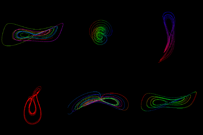 |
Newton–Leipnik Attractor — Arises from a rigid-body rotation model with a linear feedback torque; it has two coexisting scroll-shaped attractors.
dx/dt = −ax + y + 10yz
dy/dt = −x − 0.4y + 5xz
dz/dt = bz − 5xy
#newtonleipnik · 3-D flow

| Arneodo | animated |
|---|---|
 |
 |
Arneodo Attractor — Arneodo, Coullet and Tresser (1981): a third-order jerk equation, x‴ = −ax − bx′ − x″ + dx³, written as three first-order equations. A spiral attractor whose loops fold back on themselves through the cubic term.
dx/dt = y
dy/dt = z
dz/dt = −ax − by − z + dx³
#arneodo · 3-D flow

| Chen-Lee | animated |
|---|---|
 |
 |
Chen–Lee Attractor — Chen and Lee (2004): the Euler equations of a rigid body in rotation, with linear feedback added to each axis. A two-wing attractor whose wings stand on the z axis.
dx/dt = ax − yz
dy/dt = by + xz
dz/dt = cz + xy/d
#chenlee · 3-D flow

| Dequan Li | animated |
|---|---|
 |
 |
Dequan Li Attractor — Li (2008): a three-scroll attractor, the scrolls joined through the z axis. Stiff: its default step is small, and larger steps of dt make the trajectory leave the attractor.
dx/dt = a(y − x) + cxz
dy/dt = ex + fy − xz
dz/dt = bz + xy − dx²
#dequanli · 3-D flow

| Three-Scroll | animated |
|---|---|
 |
 |
Three-Scroll Attractor — the three-scroll unified chaotic system (TSUCS): the Dequan Li system without the x term in dy/dt, which opens its three scrolls wider.
dx/dt = a(y − x) + cxz
dy/dt = ey − xz
dz/dt = bz + xy − dx²
#threescroll · 3-D flow

| Wang-Sun | animated |
|---|---|
 |
 |
Wang–Sun Attractor — Wang and Sun (2010): a four-wing attractor, the trajectory passing between four lobes arranged around the z axis rather than the usual two.
dx/dt = ax + cyz
dy/dt = bx + dy − xz
dz/dt = ez + fxy
#wangsun · 3-D flow

| Lorenz Mod 2 | animated |
|---|---|
 |
 |
Lorenz Mod 2 Attractor — the second modified Lorenz system: the quadratic terms of the Lorenz equations rearranged so that the two wings fold into a single rotating body.
dx/dt = −ax + y² − z² + ac
dy/dt = x(y − bz) + d
dz/dt = −z + x(by + z)
#lorenzmod2 · 3-D flow

| Simone | animated |
|---|---|
 |
 |
Simone Attractor — a point drawn toward s·(sin(ay) + cos(bz), sin(az) + cos(bx), sin(ax) + cos(by)): the trigonometric map of the Simone attractor written as a flow, each coordinate driven by the other two. From Shashank Tomar's strange attractors. Chaotic for some (a, b) and periodic for others; b = 2.49 is chaotic.
dx/dt = s(sin(ay) + cos(bz)) − x
dy/dt = s(sin(az) + cos(bx)) − y
dz/dt = s(sin(ax) + cos(by)) − z
#simone · 3-D flow
Rucklidge Attractor — A. M. Rucklidge's 1992 model of double convection: a layer of fluid heated from below while a magnetic field or the frame's rotation pushes back. Two scrolls like Lorenz's, wound more tightly.
dx/dt = −κx + λy − yz
dy/dt = x
dz/dt = −z + y²
#rucklidge · 3-D flow
Genesio–Tesi Attractor — from Genesio and Tesi's 1992 study in control theory of when a feedback system stops oscillating regularly and turns chaotic. A jerk system: the third derivative of x set by x and its first two derivatives, with one square.
dx/dt = y
dy/dt = z
dz/dt = −cx − by − az + x²
#genesiotesi · 3-D flow
Shimizu–Morioka Attractor — Shimizu and Morioka's 1980 system, a relative of Lorenz's in which the butterfly's wings meet in a lip, a fold where the orbit hesitates before choosing a side.
dx/dt = y
dy/dt = x − λy − xz
dz/dt = −αz + x²
#shimizumorioka · 3-D flow
Rikitake Dynamo — T. Rikitake's 1958 model of the Earth's magnetic field: two disk dynamos, each feeding the other's coil. x and y are their currents, and they reverse sign at irregular times, as the geomagnetic field has reversed through geological time.
dx/dt = −μx + zy
dy/dt = −μy + (z − a)x
dz/dt = 1 − xy
#rikitake · 3-D flow
Moore–Spiegel Attractor — Moore and Spiegel's 1966 model of a parcel of gas in a star's atmosphere, rising and sinking through convection while it radiates heat away; T and R set the thermal and the buoyant forces.
dx/dt = y
dy/dt = z
dz/dt = −z − (T − R + Rx²)y − Tx
#moorespiegel · 3-D flow
Bouali Attractor — Safieddine Bouali's 2012 strange attractor with a stretched loop: a scroll with one long excursion out and back.
dx/dt = x(a − y) + αz
dy/dt = −y(b − x²)
dz/dt = −x(c − sz) − βz
#bouali · 3-D flow
Lorenz-84 — Edward Lorenz's 1984 model of the atmosphere's general circulation: x is the westerly jet, y and z the eddies that carry heat poleward, F the pole-to-equator heating and G its seasonal part. The same Lorenz, twenty years on, with weather as a whole rather than one convecting cell.
dx/dt = −y² − z² − ax + aF
dy/dt = xy − bxz − y + G
dz/dt = bxy + xz − z
#lorenz84 · 3-D flow
Finance System — Ma and Chen's 2001 model of an economy: x the interest rate, y the demand for investment, z the price index, a the saving, b the cost of investment and c the elasticity of demand. An economy can be chaotic without any shock from outside.
dx/dt = z + (y − a)x
dy/dt = 1 − by − x²
dz/dt = −x − cz
#finance · 3-D flow
Hindmarsh–Rose Neuron — Hindmarsh and Rose's 1984 model of a nerve cell: x the membrane voltage, y a fast recovery current, z a slow adaptation current, I the current injected. It fires in bursts of spikes, and at I = 3.25 how many spikes a burst has is chaotic. The slow current is slow: give it a long trail.
dx/dt = y − x³ + 3x² − z + I
dy/dt = 1 − 5x² − y
dz/dt = r(s(x + 1.6) − z)
#hindmarshrose · 3-D flow
Wei (no equilibrium) — Zhouchao Wei's 2011 system, chaotic though it has no equilibrium at all: no fixed point for the orbit to circle or be thrown from, which was long assumed to be what chaos needs. An attractor like this is hidden: it cannot be found by starting near a fixed point, because there is none.
dx/dt = −y
dy/dt = x + z
dz/dt = 2y² + xz − a
#wei · 3-D flow
Sprott Jerk — J. C. Sprott's 1997 simplest dissipative chaotic flow: x‴ = −A x″ + x′² − x, one parameter and one quadratic term. Chaotic in a narrow window of A around 2.017, from a small basin: a start outside it escapes, and the rack starts it again.
dx/dt = y
dy/dt = z
dz/dt = −Az + y² − x
#sprottjerk · 3-D flow

| Hyper-Rössler (4D) | animated |
|---|---|
 |
 |
Rössler Hyperchaos (1979) — Otto Rössler's 4-dimensional extension of his attractor, with two positive Lyapunov exponents (hyperchaos). A hidden fourth coordinate w feeds back into y; the plot is the (x,y,z) projection.
dx/dt = −y − z
dy/dt = x + ay + w
dz/dt = b + xz
dw/dt = −cz + dw
#hyperrossler · 4-D flow

| Sprott Morph | animated |
|---|---|
 |
 |
Sprott Morph — the glensstuff.com Self-Programming Analog Computer, which stepped itself through the Sprott catalog by re-patching. Every Sprott A–S system is a quadratic 3-D flow, a point in the 30-dimensional coefficient space of Sprott's 1994 search. With the rate knob up, the machine re-patches itself from one system to the next, in systems per minute, while ONE trajectory keeps integrating; the wired readout under the monitor shows the current wiring. B–S are chaotic attractors, stepped with RK4 as their own models are; A is conservative, a chaotic sea rather than an attractor. With the rate at zero the sys knob parks the patch anywhere in the cycle, including between two systems, where the coefficients are blended linearly. Most blends are not attractors: measured at quarter steps, the large majority diverge or settle onto a cycle or a fixed point, and a guard reseeds the trajectory when a blend flings it away. Coefficients are extracted numerically from the catalog's own equations.
#sprottmorph · 3-D flow
| Sprott A | animated |
|---|---|
 |
 |
Sprott A (Nosé–Hoover oscillator) — the first of J. C. Sprott's 1994 systems and the only conservative one: rather than settling onto a strange attractor it fills a chaotic sea.
dx/dt = y
dy/dt = −x + yz
dz/dt = 1 − y²
#sprotta · 3-D flow
| Sprott B | animated |
|---|---|
 |
 |
Sprott B — one of J. C. Sprott's simple chaotic flows (1994), realized as an analog circuit at glensstuff.com. Found by systematic search for the algebraically simplest systems that still produce chaos.
Five terms, two of them nonlinear (yz and xy). ∇·F = −1 everywhere, so a cloud of starting points loses volume at one steady rate, by a factor of e every unit of time. The equations are unchanged by (x, y, z) → (−x, −y, z), so the attractor is symmetric under a half turn about the z axis, or has a twin that is its half-turned copy.
dx/dt = yz
dy/dt = x − y
dz/dt = 1 − xy
#sprottb · 3-D flow
| Sprott C | animated |
|---|---|
 |
 |
Sprott C — one of J. C. Sprott's simple chaotic flows (1994), realized as an analog circuit at glensstuff.com. Found by systematic search for the algebraically simplest systems that still produce chaos.
Five terms, two of them nonlinear (yz and x²). ∇·F = −1 everywhere, so a cloud of starting points loses volume at one steady rate, by a factor of e every unit of time. The equations are unchanged by (x, y, z) → (−x, −y, z), so the attractor is symmetric under a half turn about the z axis, or has a twin that is its half-turned copy.
dx/dt = yz
dy/dt = x − y
dz/dt = 1 − x²
#sprottc · 3-D flow
| Sprott D | animated |
|---|---|
 |
 |
Sprott D — one of J. C. Sprott's simple chaotic flows (1994), realized as an analog circuit at glensstuff.com. Found by systematic search for the algebraically simplest systems that still produce chaos.
Five terms, two of them nonlinear (y² and xz). ∇·F = x, which changes sign at x = 0: volume grows where x > 0 and shrinks where x < 0, so the flow is dissipative only on average along the attractor.
dx/dt = −y
dy/dt = x + z
dz/dt = xz + 3y²
#sprottd · 3-D flow
| Sprott E | animated |
|---|---|
 |
 |
Sprott E — one of J. C. Sprott's simple chaotic flows (1994), realized as an analog circuit at glensstuff.com. Found by systematic search for the algebraically simplest systems that still produce chaos.
Five terms, two of them nonlinear (yz and x²). ∇·F = −1 everywhere, so a cloud of starting points loses volume at one steady rate, by a factor of e every unit of time.
dx/dt = yz
dy/dt = x² − y
dz/dt = 1 − 4x
#sprotte · 3-D flow
| Sprott F | animated |
|---|---|
 |
 |
Sprott F — one of J. C. Sprott's simple chaotic flows (1994), realized as an analog circuit at glensstuff.com. Found by systematic search for the algebraically simplest systems that still produce chaos.
Six terms, one of them nonlinear (x²). ∇·F = −0.5 everywhere, so a cloud of starting points loses volume at one steady rate, by a factor of e every 2 time units.
dx/dt = y + z
dy/dt = −x + 0.5y
dz/dt = x² − z
#sprottf · 3-D flow
| Sprott G | animated |
|---|---|
 |
 |
Sprott G — one of J. C. Sprott's simple chaotic flows (1994), realized as an analog circuit at glensstuff.com. Found by systematic search for the algebraically simplest systems that still produce chaos.
Six terms, one of them nonlinear (xz). ∇·F = −0.6 everywhere, so a cloud of starting points loses volume at one steady rate, by a factor of e every 1.7 time units.
dx/dt = 0.4x + z
dy/dt = xz − y
dz/dt = −x + y
#sprottg · 3-D flow
| Sprott H | animated |
|---|---|
 |
 |
Sprott H — one of J. C. Sprott's simple chaotic flows (1994), realized as an analog circuit at glensstuff.com. Found by systematic search for the algebraically simplest systems that still produce chaos.
Six terms, one of them nonlinear (z²). ∇·F = −0.5 everywhere, so a cloud of starting points loses volume at one steady rate, by a factor of e every 2 time units.
dx/dt = −y + z²
dy/dt = x + 0.5y
dz/dt = x − z
#sprotth · 3-D flow
| Sprott I | animated |
|---|---|
 |
 |
Sprott I — one of J. C. Sprott's simple chaotic flows (1994), realized as an analog circuit at glensstuff.com. Found by systematic search for the algebraically simplest systems that still produce chaos.
Six terms, one of them nonlinear (y²). ∇·F = −1 everywhere, so a cloud of starting points loses volume at one steady rate, by a factor of e every unit of time.
dx/dt = −0.2y
dy/dt = x + z
dz/dt = x + y² − z
#sprotti · 3-D flow
| Sprott J | animated |
|---|---|
 |
 |
Sprott J — one of J. C. Sprott's simple chaotic flows (1994), realized as an analog circuit at glensstuff.com. Found by systematic search for the algebraically simplest systems that still produce chaos.
Six terms, one of them nonlinear (y²). ∇·F = −2 everywhere, so a cloud of starting points loses volume at one steady rate, by a factor of e every 0.5 time units.
dx/dt = 2z
dy/dt = −2y + z
dz/dt = −x + y + y²
#sprottj · 3-D flow
| Sprott K | animated |
|---|---|
 |
 |
Sprott K — one of J. C. Sprott's simple chaotic flows (1994), realized as an analog circuit at glensstuff.com. Found by systematic search for the algebraically simplest systems that still produce chaos.
Six terms, one of them nonlinear (xy). ∇·F = y − 0.7, which changes sign at y = 0.7: volume grows where y > 0.7 and shrinks where y < 0.7, so the flow is dissipative only on average along the attractor.
dx/dt = xy − z
dy/dt = x − y
dz/dt = x + 0.3z
#sprottk · 3-D flow
| Sprott L | animated |
|---|---|
 |
 |
Sprott L — one of J. C. Sprott's simple chaotic flows (1994), realized as an analog circuit at glensstuff.com. Found by systematic search for the algebraically simplest systems that still produce chaos.
Six terms, one of them nonlinear (x²). ∇·F = −1 everywhere, so a cloud of starting points loses volume at one steady rate, by a factor of e every unit of time.
dx/dt = y + 3.9z
dy/dt = 0.9x² − y
dz/dt = 1 − x
#sprottl · 3-D flow
| Sprott M | animated |
|---|---|
 |
 |
Sprott M — one of J. C. Sprott's simple chaotic flows (1994), realized as an analog circuit at glensstuff.com. Found by systematic search for the algebraically simplest systems that still produce chaos.
Six terms, one of them nonlinear (x²). ∇·F = −1 everywhere, so a cloud of starting points loses volume at one steady rate, by a factor of e every unit of time.
dx/dt = −z
dy/dt = −x² − y
dz/dt = 1.7 + 1.7x + y
#sprottm · 3-D flow
| Sprott N | animated |
|---|---|
 |
 |
Sprott N — one of J. C. Sprott's simple chaotic flows (1994), realized as an analog circuit at glensstuff.com. Found by systematic search for the algebraically simplest systems that still produce chaos.
Six terms, one of them nonlinear (z²). ∇·F = −2 everywhere, so a cloud of starting points loses volume at one steady rate, by a factor of e every 0.5 time units.
dx/dt = −2y
dy/dt = x + z²
dz/dt = 1 + y − 2z
#sprottn · 3-D flow
| Sprott O | animated |
|---|---|
 |
 |
Sprott O — one of J. C. Sprott's simple chaotic flows (1994), realized as an analog circuit at glensstuff.com. Found by systematic search for the algebraically simplest systems that still produce chaos.
Six terms, one of them nonlinear (xz). ∇·F = x, which changes sign at x = 0: volume grows where x > 0 and shrinks where x < 0, so the flow is dissipative only on average along the attractor.
dx/dt = y
dy/dt = x − z
dz/dt = x + xz + 2.7y
#sprotto · 3-D flow
| Sprott P | animated |
|---|---|
 |
 |
Sprott P — one of J. C. Sprott's simple chaotic flows (1994), realized as an analog circuit at glensstuff.com. Found by systematic search for the algebraically simplest systems that still produce chaos.
Six terms, one of them nonlinear (y²). ∇·F = 2y, which changes sign at y = 0: volume grows where y > 0 and shrinks where y < 0, so the flow is dissipative only on average along the attractor.
dx/dt = 2.7y + z
dy/dt = −x + y²
dz/dt = x + y
#sprottp · 3-D flow
| Sprott Q | animated |
|---|---|
 |
 |
Sprott Q — one of J. C. Sprott's simple chaotic flows (1994), realized as an analog circuit at glensstuff.com. Found by systematic search for the algebraically simplest systems that still produce chaos.
Six terms, one of them nonlinear (y²). ∇·F = −0.5 everywhere, so a cloud of starting points loses volume at one steady rate, by a factor of e every 2 time units.
dx/dt = −z
dy/dt = x − y
dz/dt = 3.1x + y² + 0.5z
#sprottq · 3-D flow
| Sprott R | animated |
|---|---|
 |
 |
Sprott R — one of J. C. Sprott's simple chaotic flows (1994), realized as an analog circuit at glensstuff.com. Found by systematic search for the algebraically simplest systems that still produce chaos.
Six terms, one of them nonlinear (xy). ∇·F = −1 everywhere, so a cloud of starting points loses volume at one steady rate, by a factor of e every unit of time.
dx/dt = 0.9 − y
dy/dt = 0.4 + z
dz/dt = xy − z
#sprottr · 3-D flow
| Sprott S | animated |
|---|---|
 |
 |
Sprott S — one of J. C. Sprott's simple chaotic flows (1994), realized as an analog circuit at glensstuff.com. Found by systematic search for the algebraically simplest systems that still produce chaos.
Six terms, one of them nonlinear (z²). ∇·F = −1 everywhere, so a cloud of starting points loses volume at one steady rate, by a factor of e every unit of time.
dx/dt = −x − 4y
dy/dt = x + z²
dz/dt = 1 + x
#sprotts · 3-D flow

| Custom equation | animated |
|---|---|
 |
 |
Custom Equations — type your own system. The Equation module takes dx/dt, dy/dt and dz/dt (plus dw/dt for a 4-D system) as text and integrates them with forward Euler, the same way the classic attractors are stepped. The iter switch under the monitor reads the same expressions as a discrete MAP instead — x = f(x,y,z) rather than x += dt·f(x,y,z) — which has no dt and no path between iterates, so it draws as a cloud of points the way Henon and Ikeda do.
There is no eval: expressions are tokenized, converted to RPN and interpreted over a small value stack, so nothing but arithmetic can run. Grammar is + − × ÷ ^ with grouping and implicit multiplication (2x, 3(x+1)), the functions sin cos tan asin acos atan exp log ln sqrt abs sign sinh cosh tanh floor, the constants pi e tau, and the variables x y z w t. Any other name becomes a free parameter and is auto-exposed as its own knob.
#custom · 4-D flow
Henon · Ikeda · Clifford · Peter de Jong · Gumowski-Mira · Tinkerbell · Chirikov Standard Map · Bifurcation · Poincaré Section

| Henon | animated |
|---|---|
 |
 |
Hénon map (M. Hénon, "A two-dimensional mapping with a strange attractor", 1976) — the example that showed a strange attractor needs neither a flow nor three dimensions, only a stretch and a fold. Zoom in anywhere on a filament and it resolves into more filaments: locally a line crossed with a Cantor set. Its Jacobian determinant is −b, so area contracts by exactly b every iterate no matter where you are.
x' = 1 − a·x² + y
y' = b·x
#henon · discrete map

| Ikeda | animated |
|---|---|
 |
 |
Ikeda map (K. Ikeda, 1979) — light circulating in a nonlinear optical cavity, where each pass rotates the complex field by an amount that depends on its own intensity. That intensity-dependent rotation is the whole mechanism: the more energetic part of the beam turns further, and the attractor's hook is the result.
t = 0.4 − 6/(1 + x² + y²)
x' = 1 + u·(x·cos t − y·sin t)
y' = u·(x·sin t + y·cos t)
#ikeda · discrete map

| Clifford | animated |
|---|---|
 |
 |
Clifford attractor (Clifford Pickover) — a trigonometric map with no physical derivation, kept because of what it draws. Every parameter change reshapes it entirely, which makes the four knobs worth turning slowly.
x' = sin(a·y) + c·cos(a·x)
y' = sin(b·x) + d·cos(b·y)
#clifford · discrete map

| Peter de Jong | animated |
|---|---|
 |
 |
Peter de Jong attractor — the same idea as Clifford's with the terms paired differently, and a different family of figures for it. Four knobs, an enormous space of shapes, and no way to predict which you will get.
x' = sin(a·y) − cos(b·x)
y' = sin(c·x) − cos(d·y)
#dejong · discrete map

| Gumowski-Mira | animated |
|---|---|
 |
 |
Gumowski-Mira map (I. Gumowski and C. Mira, CERN, 1980) — written to study how a particle beam drifts turn after turn around an accelerator ring, and it produces organic, almost biological figures that look nothing like their origin. The shared nonlinearity g is applied twice per iterate, to x and then to the NEW x. Unlike the others here it is QUASI-PERIODIC at these settings rather than chaotic: the curves it draws are invariant curves the orbit winds around forever, not a fractal dust. Two orbits started a hair apart drift apart slowly instead of separating exponentially, which is why the figure looks woven rather than sprayed.
g(v) = μ·v + 2(1−μ)·v²/(1+v²)
x' = y + a(1 − b·y²)·y + g(x)
y' = −x + g(x')
#mira · discrete map

| Tinkerbell | animated |
|---|---|
 |
 |
Tinkerbell map — a quadratic map of the plane whose orbit sweeps a curved, wing-like region. Bounded only for a narrow band of parameters; push the knobs and it escapes to infinity, which the renderer catches and reseeds rather than drawing NaNs.
x' = x² − y² + a·x + b·y
y' = 2·x·y + c·x + d·y
#tinkerbell · discrete map

| Chirikov Standard Map | animated |
|---|---|
 |
 |
Chirikov standard map (B. Chirikov, 1979) — the canonical AREA-PRESERVING map, and the one system here with no attractor at all. A kicked rotor: each iterate kicks the momentum by K·sin θ and lets the angle advance. Because area is preserved nothing contracts onto anything, so it is drawn as an ensemble of orbits rather than one — a single orbit would trace its own invariant curve and tell you nothing about the rest. Turn K up and watch the intact curves break into a chaotic sea with islands of stability stranded in it; near K ≈ 0.9716 the last curve spanning the phase space goes, and orbits can wander in momentum without bound.
p' = p + K·sin θ
θ' = θ + p'   (both mod 2π)
#standardmap · discrete map

| Bifurcation | animated |
|---|---|
 |
 |
Bifurcation Explorer — the fig-tree diagram, computed live. One parameter of the most recent flow mode sweeps its whole knob range across the x axis; each column integrates the system fresh at that value and plots the local maxima of z. Thin branches are periodic orbits, fan-outs are period-doubling cascades, filled bands are chaos — the route between them is the route to chaos. Pick the swept parameter on the sweep selector in the model bank, with drive beside it; visit an attractor and tune it to change the source system.
#bifurcation · parametric

Poincaré Section — the continuous flow read as a discrete point set. The most recent flow mode is integrated privately and sampled only where it pierces a plane, going one way through it; what is left is the cross-section of the attractor, and the sheets that are invisible in the tangle are the whole picture here.
AXIS and POS place the plane (POS is a fraction of the attractor's own reach along that axis, so 0 is through the middle whatever the system's size); DIR chooses which way through it counts. One way is the default, and it is not a preference: a bounded flow that goes up through a plane has to come back down through it, so keeping both superimposes two different sections and the return map stops being a function.
VIEW picks the picture — PLANE draws the crossings where they physically are, FLAT lays the section out face on in the plane's own coordinates, and MAP is the FIRST-RETURN MAP: each crossing plotted against the next one. That last is where the route to chaos is legible — a periodic orbit is a handful of dots, a period-doubling is that set doubling, and a chaotic attractor is a single-humped curve, which is the logistic map's parabola surfacing inside a differential equation. The dotted 45° line is y = x, where the map's fixed points are.
The crossing point is INTERPOLATED between the two samples that straddle the plane rather than snapped to the nearer of them — snapping smears the section by up to half a step of arc, which on these attractors is the same size as the gap between the sheets it is supposed to show.
The same section is available as an overlay on any flow: the S button on LINE (Display), or ON on AXIS in the model bank.
#poincare · parametric
STL File · Terminal · Terminal Animation · Host Shell · Desk · Lattice

| STL File | animated |
|---|---|
 |
 |
STL File — Load a stereolithograph (.stl, binary or ASCII) from disk with the load switch under the monitor and it renders as a rotating wireframe. Very large files are decimated to fit the 16-bit index pipeline.
#stlfile · geometry
Terminal — a live terminal, drawn as a model.
It is the same texture-on-a-plane path the spectrogram and the recurrence plot use, so it rotates, zooms and takes a gradient like any other model;
what is on the texture is xterm-go (https://github.com/0magnet/xterm-go), a Go port of xterm.js, rendering a real terminal grid with WebGL2.
That last part is what makes this possible rather than merely desirable: a terminal drawn as DOM could not be sampled into a texture at all, and rasterizing DOM every frame is not a thing worth doing.
xterm-go renders into a canvas, and a canvas is a texture source.
Behind it runs websh (https://github.com/0magnet/websh), a Bash interpreter compiled to wasm over an in-memory filesystem, so this is a session you can work in and not a picture of one: pipes, globs, redirection, for loops, all of it rotating with the model.
Double-click the canvas to type into it and Esc to give the keyboard back — a double click because a single one is how you rotate the model, and the two must not be the same gesture.
Focusing it silences the app's own key bindings automatically, since Pong, the Keys module and the hovered-knob arrows all already stand aside for a focused textarea, which is what a terminal captures keys on.
It can also be the BACKDROP behind another model, the way the spectrogram can.
#terminal · geometry

Terminal Animation — the same terminal-on-a-plane, with a drawing program on it instead of a shell. The catalog is tuiwasm (https://github.com/0magnet/tuiwasm): animations — fire, plasma, a matrix rain, an aquarium, a bonsai growing branch by branch, Langton's ant, falling sand — plus charts, tables and styled text. Pick one from the prog selector on this model's panel. The animations draw at half-block resolution: every cell is an upper or lower block glyph carrying its own foreground and background, which is two independently colored pixels per cell and roughly square ones, since a terminal cell is about twice as tall as it is wide. They run at the frame rate — the cells are written straight into xterm-go's buffer rather than encoded as escape sequences and parsed back, which is the difference between sixty frames a second and a wedged tab. Nothing is wired to the keyboard here, unlike the Terminal model: these draw, they do not read, and the animations quit on a keystroke. Like the terminal it can also be the BACKDROP behind another model.
#termanim · geometry
Host Shell — a real shell on the machine serving this page, drawn as a model. The Terminal model beside it is websh (https://github.com/0magnet/websh), a Bash interpreter compiled into the wasm over a filesystem that exists only in the browser; this one is a pty on the host, reached through the same agent the desk's host pane uses. It needs the server to have been started with --shell, which also forces a loopback bind — the server refuses that flag on a listener the network can reach rather than warning about it. Without the flag the terminal still opens and says so, because an empty rectangle with no explanation is the worse answer. Double-click the canvas to type into it and Esc to give the keyboard back, exactly as for the Terminal model. It reached the screen before this as a window inside the Desk; as a model it is the shell without the window manager around it.
#hostterm · geometry

Desk — a window manager, drawn as a model. The same texture-on-a-plane path the spectrogram, the recurrence plot and the Terminal use, with a whole desk (https://github.com/0magnet/desk) on it: winbox windows, a websh (https://github.com/0magnet/websh) shell in each, a file manager, all of them running while you rotate them.
It needed something from desk to be possible at all. A window is more than its pane — its title, buttons and border are DOM, and DOM cannot be sampled into a texture — so texturing the panes alone would give a desk of frameless rectangles. desk's WebGL compositor can now REDRAW the frames instead: each title bar is rasterized with Canvas2D, text and buttons and all, into the same canvas it draws the panes into, and that canvas is a complete picture of the desk.
Nothing types into it while it is a model, and that is the arrangement rather than an omission for the MOUSE: a click on a rotated quad would have to be cast through it to a texture coordinate and synthesized back into a DOM event at a place nothing is. What you get instead are two gestures. Ctrl-drag reaches the desk, so ctrl-dragging a title bar moves a window while an ordinary drag still turns the model; the pass switch under the monitor (Pass-through) swaps the two if you would rather drag windows directly and hold ctrl to turn. And the KEYBOARD does reach it: double-click the canvas to type into the focused window and Esc to give the keyboard back, the same pair the Terminal and Host Shell models use.
Aiming is the honest limitation — you are pointing at a projection, so a title bar is not where the pointer says it is. The Desk switch (Console → Rack) puts the same windows on the page as ordinary DOM, which is the one to use for arranging them; rearrange there, then come back here to look at it. Flatten to work, rotate to admire. It can also be the BACKDROP behind another model, the way the spectrogram and the terminal can.
#desk · geometry

Lattice — a solid drawn in depth by terminals. lattice (https://github.com/0magnet/lattice) is an ordinary terminal program that draws one cross-section of a turning solid in characters. Here 3N copies of it run, each in a terminal of its own, and the terminals are stacked as transparent sheets: N across each axis, three families each perpendicular to the other two. Whichever way the stack is turned, one family faces you and the other two are edge on, so the solid has depth from every side, and each family is brightened as it comes face on and dimmed as it goes edge on, so the solid stays as bright as it turns.
The terminals are real: each is xterm-go's emulator, and each program writes into it the same escape sequences it writes into any terminal. Only the drawing is the rack's, every character on a clear sheet, because a cell at the default background is clear, as it is in a translucent terminal. Seen from behind, a sheet reads mirrored, as glass does.
The solid is turned by the time of day, not by the rack: lattice -axis z -slice 6 in a real terminal of 24 columns by 12 rows beside the page draws the same slice at the same moment, because a terminal's size is the resolution — zoom it out and it draws a finer one.
Its cells in bay 1 are how the sheets are drawn: their rows, style, look, opacity, which families there are and what the view turns. SRC, the first of them, chooses what is drawn: one of the lattice's own solids, or any other model, drawn the same way from its trail, mesh or dots while it runs as itself, its constants in the bank beside the lattice's. The Turtle is the exception that fits: it walks the same integer grid, so without weight it is drawn from its walk rather than its trail, every step a whole number of voxels (or every voxel a whole number of steps) along an axis, and every corner the end of a straight run.
#lattice · geometry
Polyhedron · Nested Cube · Globe · Torus · Magnetosphere
| Polyhedron | animated |
|---|---|
 |
 |
Polyhedron — The regular solids and tilings, by Schläfli symbol {p,q}: faces of p sides, q of them at every corner. {3,3} is the tetrahedron, {4,3} the cube, {3,4} the octahedron, {5,3} the dodecahedron, {3,5} the icosahedron; where the corners make a full turn the faces tile the plane, and past it they tile the hyperbolic plane, drawn in Poincaré's disk. On a solid, morph cuts the corners through the rectified solid to the dual, op applies a Conway operator and kis raises a pyramid on every face.
#polyhedron · geometry
| Nested Cube | animated |
|---|---|
 |
 |
Nested Cube — A cube within a cube, two separate wireframes, illustrating the relationship between inner and outer geometric structures.
#nestedcube · geometry

| Globe | animated |
|---|---|
 |
 |
Globe — A wireframe sphere showing lines of latitude and longitude, similar to the graticule on a geographic globe. Latitude lines are horizontal circles parallel to the equator, longitude lines are great circles passing through the poles.
#globe · geometry

| Torus | animated |
|---|---|
 |
 |
Torus — A doughnut-shaped surface of revolution generated by revolving a circle (radius r) around an axis at distance R from the center of the circle.
#torus · geometry
| Magnetosphere | animated |
|---|---|
 |
 |
Magnetosphere — A visualization of magnetic field lines surrounding a dipole, similar to Earth's magnetosphere that shields the planet from solar wind.
#magnetosphere · geometry

| Turtle Path | animated | in 2-D (mod 30, closed) |
|---|---|---|
 |
 |
 |
Turtle Path — Reduce an integer sequence modulo m and the remainders repeat; the length of the repeat is the Pisano period. Read each term as an instruction — odd turns left and steps forward, even turns right and steps forward, zero does neither — and the walk draws a figure.
In three dimensions the parity of the NEXT term decides whether the turn is a yaw or a pitch, which is not arbitrary: the pair (F_n, F_n+1) mod m is the state of the recurrence, and the Pisano period is the period of that pair. One pass decides the rest, without walking further: the figure either closes, drifts in a straight line, or screws away along an axis.
The walk never finishes and is never restarted — the turtle is held mid-stride and extended at the Speed knob's rate, forever, and TRAIL is how much stays behind it (whole, long, short, comet) as the oldest scrolls off the far end.
CAM is where it is watched from. Only follow cares where the head is; every other setting places the figure by its DRIFT, the one direction it is going overall, known exactly from one pass of the period rather than guessed at from the last few frames — and for a screw it centers on the axis the classification locates, so the figure turns on the spot instead of swinging around it. fit then only decides how big it is drawn, lock holds that size too, and auto fits a closed figure and locks one that drifts.
TINT is what a color means — step, pass, visits, heading, turn, term, age — and set SRC on Layers · Colors to trail to see it, or leave it on X/Y/Z to read position instead (a flat DIM 2 figure has no Z to follow).
MUL multiplies the Fibonacci sequence, CAP limits the terms read for sequences that may not repeat, CYCLE steps to the next modulus every so many seconds, and MOD 0 draws the sequence unreduced.
Physics gives the figure weight, with ON on GRAV, the first of its four positions in the model bank after the Turtle's own: it becomes a rigid body in the plane of the screen — three degrees of freedom, the figure's own shape as its mass — inside a solid box the size of the frame, where GRAV (either way up), FRIC, BOUNCE and SPIN say how it behaves. Press on the figure and you can pick it up and throw it; press beside it and you are turning the view as usual. The walk keeps extruding while it lies there, new points arriving at the head and old ones dropping off the tail, so the figure slides through its own body and marches. Switched off, CAM places the figure again.
#turtle · parametric
Lissajous · Graphic Artist · Scope Pong · Fourier Text · Scope Clock · Bouncing Ball · XY Scope

| Lissajous | animated |
|---|---|
 |
 |
Lissajous Curve — Named after Jules Antoine Lissajous (1822–1880), these are parametric curves formed by combining sinusoidal motions along each axis. Not a chaotic system — the curves are periodic and their shape depends on the frequency ratios and phase relationships between the three oscillations.
x(t) = sin(at)
y(t) = sin(bt)
z(t) = sin(ct)
#lissajou · parametric

| Graphic Artist | animated |
|---|---|
 |
 |
Graphic Artist — a digital re-creation of Mitchell Waite's "Oscilloscope Graphic Artist" (Popular Electronics, November 1975), which drove a scope's X/Y inputs with harmonically related signals to draw 3-D-looking wireframes. Four relaxation oscillators A/B/C/D, each square or triangle: A is the fixed master and B/C/D lock to it at integer harmonics — the sync the original circuit was meant to enforce, and which a wiring error on real builds defeated, leaving them drawing an unstable blur. Carrier C is split ±45° and the B envelope modulates each phase; the two perpendicular components are what create the volume illusion on a flat scope, and here that component is lifted onto a real Z so the figure genuinely has depth.
VERT = levelA·A + levelB·(B · C₊₄₅)
HORIZ = levelD·D + levelB·(B · C₋₄₅)
#graphicartist · parametric

| Scope Pong | animated |
|---|---|
 |
 |
Scope Pong — An homage to the glensstuff.com analog Oscilloscope Pong: the whole game is one multiplexed beam tour driving the X/Y inputs, so the court, net, score ticks, paddles and ball share a single stroke — the faint diagonal beams are the retrace an unblanked scope really shows.
W / S move the left paddle, ↑ / ↓ the right; a side left alone for ~10 s returns to the machine player (it boots as a self-playing demo). The match starts over when a side passes 9, or at once with the rset switch under the monitor. Knobs: speed (the ball's), paddle (its size), skill (the machine player's), and left and right, the two paddle pots.
#pong · parametric

| Fourier Text | animated |
|---|---|
 |
 |
Fourier Text — An homage to the glensstuff.com Fourier Synthesis Character Generator, which built alphanumerics on a scope from summed harmonics. The banner's whole beam tour (strokes and retrace jumps alike) is one complex periodic signal x(t)+i·y(t); what's drawn is its reconstruction from only the first N harmonics — real harmonic synthesis, not a blur. One harmonic is an ellipse, so at low N the letters melt into loops; raise the harm knob and overtones sharpen them into legibility. Type the banner in the text field on the line under the monitor (Visual bay); Model Out plays the actual harmonic stack.
#scopetext · parametric
Scope Clock — the time, drawn the way a scope draws anything: as ONE beam tour. The face, the twelve ticks and the three hands are a single path walked in order, because an X/Y display has one beam and no way to lift it — so the jumps between the end of one stroke and the start of the next are drawn too, and show as the faint diagonals an unblanked scope really shows. Scope Pong and the Fourier banner are built the same way; this is the same instrument told the time.
The beam is spaced evenly along the whole path rather than given a fixed number of points per stroke: the face is a full circle and a tick is a few hundredths of one, so per-stroke spacing would put most of the beam on the ticks and leave the circle dotted. Even spacing is also what a real scope does, since the beam moves at a rate rather than at a number of samples.
The hands are fractional throughout — the hour hand creeps with the minutes, the minute hand with the seconds — because a clock whose hands jump looks stopped in between. TRAIL and Persist apply as they do to any trace, so a long trail smears the second hand into a comet.
#scopeclock · parametric

| Bouncing Ball | animated |
|---|---|
 |
 |
Bouncing Ball — The classic analog-computer demo (Telefunken shipped it to sell integrators): two integrator chains under constant gravity, a comparator that flips the vertical velocity at the floor with a restitution loss, and wall reflections for the drift. The scope draws the familiar train of shrinking parabolic arcs; when the bounces decay away the machine re-kicks the ball, as the unattended trade-show loop did. Floor hits blip at a pitch set by impact speed (once audio is unlocked by any interaction). Knobs: grav, bounce (the restitution), drift and height; the drop switch under the monitor lets the ball go again from that height. Try Persist to paint the full arc family.
y'' = −g, bounce: v ← −e·v at the floor
#bounceball · parametric

| XY Scope | animated |
|---|---|
 |
 |
X/Y Scope — the classic two-channel oscilloscope figure, drawing the live audio's (left, right) sample pairs as a line strip. This is the goniometer, or stereo vectorscope, that sits on a mastering desk: correlated channels lie on a diagonal, anti-correlated on the other, and a phase difference opens the diagonal into an ellipse — which is how the display doubles as a stereo phase meter and a mono compatibility check, since what lies along the anti-correlated diagonal is exactly what disappears when the mix is summed to mono. The deflection is squared against the shorter side of the window, so the mono diagonal reads at 45° and a quarter-cycle phase difference draws a circle — not an ellipse the window's shape put there. An angle that cannot be trusted is the one thing a phase display may not have. A mono source is plotted against a lagged copy of itself, since a raw mono signal would otherwise be a featureless diagonal; the Stereo Embedding next door is the same figure with a third axis, and it does not fake a channel that is not there.
AXES turns the display 45° into mid/side — M=(L+R)/2 and S=(L−R)/2, the orientation broadcast goniometers ship in, where center content lies along one axis and difference content along the other, so width is an extent rather than the eccentricity of a tilted ellipse.
GAIN is the deflection; WIN the time base in milliseconds, short for the instantaneous phase relationship and long for the width of a whole mix; GLOW the afterglow, which is the control a hardware vectorscope is actually used through — at zero the frame is cleared as it always was, above it the trace decays instead, so a transient leaves something to read. LAG is how far a mono source is delayed against itself and SMTH how hard the beam is slew-limited between samples.
CORR is the correlation meter: +1.00 means the channels are identical and the figure is the diagonal line, 0 means unrelated and a round cloud, −1.00 means one is the other's polarity inverted — which is exactly the content that disappears when the mix is summed to mono, and the reason this display is a mono-compatibility check. It reads L against R whatever AXES is set to, because it is a property of the channels rather than of the way they are drawn.
#xy · audio
Takens Embedding · Stereo Embedding · Polar Embedding

| Takens Embedding | animated |
|---|---|
 |
 |
Takens Delay Embedding — attractor reconstruction from a single signal (F. Takens, "Detecting strange attractors in turbulence", 1981). Each trail point is the delay vector (s(t), s(t−τ), s(t−2τ)) of the live audio: a pure tone draws a closed loop, music and speech trace the geometry of whatever produced them.
τ is the embedding delay, counted in samples at a fixed 48 kHz reference so that one knob position is one DURATION — the same delay whether the sound is arriving from a 48 kHz microphone or a 24 kHz server feed, which is what it was not when the number was read as raw samples of whatever happened to be playing. The default of 72 is 1.5 ms; the MEAS readout says what the current setting is in milliseconds.
MEAS measures τ rather than guessing it: the first minimum of the signal's average mutual information (Fraser & Swinney 1986), reported beside the false-nearest-neighbor embedding dimension m (Kennel et al. 1992). It also runs BY ITSELF, once, as soon as the mode has enough audio to measure — and again if the source is swapped, because τ is a property of what is playing. Once is the whole of it: nothing here re-tunes itself per frame, because a knob that moves with the music makes the figure move with it. Press the button to measure again, or turn the knob and it stays where you put it. An m above 3 means the trail you are looking at is a projection of a higher-dimensional reconstruction.
SRC picks which signal of the live pair is embedded. Takens' theorem takes ONE observable and this is the choice of which: the mix, either channel on its own, mid, or SIDE — what the two channels do not have in common, which on a real mix is the reverb and the room rather than the instruments, and which reconstructs a different manifold from the same recording.
WIN is how much time the figure spans, in milliseconds — short is live and legible, long draws a denser tangle that turns over more slowly; GAIN sets how large a full-scale sample draws. The scale is fixed — nothing auto-ranges, so quiet passages draw small and loud ones large, and the view never moves under you; the camera is fitted once to what full scale can reach, so peaks stay on screen.
SMTH is the beam smoothing between samples, and it is the trade between how much WINDOW is on screen and how smooth the line is, since both come out of one vertex budget: at 1 the figure is raw chords through four times as many samples, which is what to use to see a long window; at 16 it is a glass-smooth beam through a short one. A straight line from one delay vector to the next is a chord, and chords are the hard corners you can see — an artifact of the drawing, not something in the signal. The same knob serves the stereo and polar embeddings.
Audio is the rack's own signal: whatever the Mixer pins to RACK L and R, which at power-up is the capture (the microphone or a server feed), and can be the generators and the instruments.
#takens · parametric

Stereo Embedding — the Takens trail built from the two channels instead of one channel's past. Takens' theorem manufactures the missing axes out of a signal's own history because there is only one signal; a stereo source has already measured two, so this mode plots them against each other and what you see is the real relationship between the channels — phase, polarity, correlation, width — rather than a reconstruction. Looked at head-on it is the goniometer (vectorscope) of a mastering desk, which is the XY Scope's figure; the third axis is what a scope with two deflection plates cannot give you.
AXES picks the assignment. L,R,L(t−τ) is the goniometer with a delay coordinate for depth: a tone that draws one ellipse edge-on unrolls into a helix, and τ still means what it means in the Takens mode. L,R,time sweeps the figure along a ribbon so successive cycles stack instead of overwriting — the only way to see a slow phase drift, which on a flat display just wobbles. The mid/side positions rotate the basis 45°: M=(L+R)/2 and S=(L−R)/2, so center content lies along one axis and difference content along the other and width is an extent rather than a tilt. τ is inert on the two 'g' positions, which have time on the third axis.
CORR is the correlation meter: +1.00 means the channels are identical and the figure is a diagonal line, 0 means they are unrelated and it is a round cloud, −1.00 means one is the other inverted (and the difference vanishes if the mix is summed to mono). A mono source reads "mono" and draws the diagonal, which is the correct picture of a signal with no stereo information in it — nothing here fakes a second channel out of a delayed copy of the first, because that delayed copy is exactly what this mode exists to stop pretending is a channel. The mid/side positions are the ones worth turning to then: S is zero and what is left is an honest two-coordinate delay embedding.
ALGN is an inter-channel DELAY, ±2 ms, and it is the fault a goniometer gets reached for: a spaced pair of microphones, a mis-clocked converter, a plugin reporting its latency wrong. An offset draws as a figure that opens into an ellipse and rotates as the frequency moves; dial the knob until the figure collapses back onto the diagonal and it reads how far apart the channels were. WIDE scales side against mid — the width control of a mid/side processor, applied to the drawing rather than to the audio, so it answers what widening would do and what would collapse if the result were summed to mono. Neither moves CORR, which goes on reading the source as it actually is.
WIN is how much time the figure spans, in milliseconds — a phase display is read over a few tens of them, past a couple of hundred it is a filled blob; GAIN sets how large a full-scale sample draws, and as in the Takens mode the scale is fixed and nothing auto-ranges.
Audio is the rack's own signal: whatever the Mixer pins to RACK L and R, which at power-up is the capture (the microphone or a server feed), and can be the generators and the instruments. The feed asks the capture for the source as it was recorded, over the WebSocket and over WebTransport alike, so a stereo sink gives real stereo either way; a server or a device with only one channel to give reads "mono".
#stereo · parametric

Polar Embedding — the Takens delay vector drawn in a sphere instead of a cube. The Takens mode plots (s(t), s(t−τ), s(t−2τ)) coordinate by coordinate, and each coordinate is one sample bounded to ±1 and multiplied by GAIN, so the reachable set is a cube: loud passages pile up against its faces and hardest of all against its corners, where all three coordinates peak together. That box is an artifact of writing the vector down in coordinates; nothing in the sound knows about the axes.
Here the vector is split into a direction and a length, the direction is kept exactly as it is, and only the length is passed through a curve that cannot exceed 1 — so the figure is bounded by a sphere, which looks the same from every angle, and no rotation finds an edge that is really the arithmetic showing through. The angles between successive delay vectors are untouched, which matters: those angles are the reconstructed geometry Takens' theorem is about, and a map that bent them would be drawing a different manifold.
MAP picks the curve. tanh is the soft clipper: near-linear when it is quiet, asymptotic to the surface when it is loud. Algebraic (soft on the ring) reaches the same surface more slowly, so the mid-range keeps more of its dynamics. dB makes the radius a level in decibels, full scale at the surface and DRV setting how many decibels down the center is (2 is 40 dB, about a level meter's useful range), so quiet program material is drawn at a size it can be read at. Direction only (unit) throws the loudness away completely and puts every point on the surface — what is left is the angular motion the amplitude was hiding, so a figure that merely swelled and shrank before now moves. DRIVE is how hard the signal is pushed into the curve, and it does nothing on the direction-only position, where there is no length left to compress.
SRC picks which signal of the live pair is embedded, as in the Takens mode. τ and WIN mean exactly what they mean in the Takens mode, and the scale is fixed there too — nothing auto-ranges, so quiet draws small and loud draws large. The camera is fitted once to the sphere, which is the whole of what a bounded radius can reach, so peaks stay on screen without the room the cube's corner needed.
Audio is the rack's own signal: whatever the Mixer pins to RACK L and R, which at power-up is the capture (the microphone or a server feed), and can be the generators and the instruments.
#polar · parametric
Spectrogram · FVF Wobbulator · Recurrence Plot · RTA — Octave Bands · Transfer Function · Waterfall — Spectral Decay
| Spectrogram | animated |
|---|---|
 |
 |
Spectrogram — a scrolling short-time Fourier transform of the live audio: frequency up the plane, time scrolling right to left, magnitude as color. It is a display inspired by Vanya Sergeev's audioprism, written in Go (github.com/0magnet/audioprism-go) and drawn here as a texture on a plane in the same 3-D pipeline as every other model, so it rotates and zooms like one — and the same texture can be painted onto other geometry with the skin switch. Its controls in the model bank expose the whole chain: transform size, overlap, window function, channel, magnitude scale and limits.
#spectrogram · audio

| FVF Wobbulator | animated |
|---|---|
 |
 |
FVF — Harmonic Wobbulator. A software analog of the Frequency→Voltage→Frequency converter with balanced modulator designed at bunkerofdoom.com (hardware built 1984). The live audio's pitch is tracked, scaled/offset into a new carrier frequency, and ring- or AM-modulated back by the original signal — the metallic, glitchy 'very strange' timbre. Shown here as the processed spectrogram.
#fvf · audio

| Recurrence Plot | animated |
|---|---|
 |
 |
Recurrence Plot — the picture of when a signal returns to where it has already been (J.-P. Eckmann, S. O. Kamphorst and D. Ruelle, "Recurrence Plots of Dynamical Systems", 1987). Time runs along both axes, and the cell (i, j) is lit when the two samples are within ε of each other, so the main diagonal is always lit and everything else says how the signal repeats. A steady tone draws unbroken diagonals spaced by its period; a chaotic or noisy source breaks them into short segments; a held sound is a solid block, and the instant the source changes is an edge running across the square.
SRC picks what is being plotted: audio is the raw samples, embed is the Takens delay vector (s, s−τ, … s−(m−1)τ) of that same audio — the reconstructed phase space a recurrence plot is properly defined on, which removes the anti-diagonals a scalar signal shows because sin t equals sin(T/2 − t) — and traj is the most recent attractor's own trajectory, the way the Bifurcation explorer picks its system. τ is the Takens mode's own τ knob, so its MEAS button measures the delay for this plot too, and m is the embedding dimension.
WIN is how much history the square covers: milliseconds for the audio sources, tenths of that in the system's own time units for a trajectory. ε is the threshold as a fraction of the source's scale — full scale for audio, the attractor's own diameter for a trajectory, which is what makes one default readable across systems that differ in width by fifty times. It is never taken from the current level, deliberately: a threshold that follows the music makes the plot's density pulse with it instead of describing it.
RQA reads the picture back as three numbers — RR, the percentage lit and the number to turn ε by; DET, the share of that lying on diagonals, which is what separates a system from noise; and LAM, the share on verticals, which is states it sat in rather than passed through. Drawn as a texture on a square plane in the same 3-D pipeline as every other model.
#recurrence · audio

RTA — Octave Bands. The real-time analyzer a room is measured with: the spectrum split into fractional-octave bands and shown as a bar per band. A spectrogram shows every bin, which is right for watching sound move and wrong for asking what a room is doing to it — linearly spaced bins put nine-tenths of the picture above 2 kHz and squeeze the bass into a few pixels. Bands of equal RATIO drawn at equal widths is a logarithmic frequency axis, which is how hearing is organized and how every acoustics standard reports.
BAND picks the width: 1/1 is a hi-fi graphic equalizer's ten, 1/3 is what room measurement and ISO use, and the two finer settings find a single narrow resonance — a 1/12-octave band is about 6% wide, roughly the ear's own resolution in the midrange. The centers are the standard ones (ISO 266 / ANSI S1.11, the base-ten series), so a reading here is comparable with anybody else's.
FEED IT PINK NOISE from a generator's pink wave: fractional-octave bands get wider in hertz as they go up, so equal power per octave is what reads FLAT — a flat display on pink noise is the definition of a flat system, and it is the convention room measurement is done in. White noise rises 3 dB per octave on the same display, which is the difference between the two and the reason pink is the one used.
TOP and RNGE place the scale in dBFS; AVG is the meter's averaging, quick to rise and slow to fall as every level meter is; HOLD is the peak-hold decay in dB per second, which is what makes the display readable on music rather than only on noise — music excites part of the band at a time and the held peaks are the envelope that accumulates into the answer. SRC picks the channel.
#rta · audio

Transfer Function — what the thing between two channels did to the sound. Every other measurement here asks about ONE signal; this one asks about the RELATIONSHIP between two, which is the question a system is actually tuned by. Send a signal into a loudspeaker, a room, a filter or a cable, capture what comes back, and read what happened in between. That is what a system-tuning rig does, and chaosrack already carries two channels end to end.
MAGNITUDE is the frequency response in dB — flat is a system that changed nothing. PHASE is how far the output lags the input; a pure DELAY is a phase that falls linearly with frequency, and the slope IS the delay, which is what the DLY readout fits and what gets dialed into a delay line to line a speaker up. COHERENCE is the number that says whether to believe the other two: 1 means the output is fully explained by the input, and noise, a second source, a nonlinearity or a system that moved during the measurement all drive it down. A dip in the magnitude with the coherence still high is the system; the same dip with the coherence collapsed is the measurement giving up, and the curves are drawn together so the two can be told apart.
AVERAGING IS NOT OPTIONAL. From a single window coherence is exactly 1 at every frequency — for any two signals whatever, including two unrelated noises — so a display built on one window is a row of perfect scores that means nothing. AVG sets how many windows are folded in before the result is shown, and the curves are drawn only where the coherence clears COH and the stimulus actually reached the band.
REF says which channel is the reference, BAND how finely the bands are smoothed, RNGE the magnitude scale, SHOW which curves are drawn. Feed it pink noise or the log sweep from a generator (its pink and swp waves).
#xfer · audio

Waterfall — Cumulative Spectral Decay. The measurement a loudspeaker is characterized by, and the one display here that could only exist in this app: every other analyzer draws its own flat panel and this is a genuine 3-D surface, so it rides the same pipeline the attractors do and drags, rotates, zooms and takes the gradient like any other model. Frequency runs left to right, logarithmically, because hearing is organized in ratios; level runs up; and TIME runs into the screen. Each line is the spectrum of what is left of the impulse response from a moment onwards, so a flat loudspeaker's surface falls away evenly and a RESONANCE is a ridge running back into the screen at one frequency. That is what this is for: a frequency response cannot tell a resonance from a broad lift, because they are identical in magnitude and nothing alike in time.
Feed it a generator's log sweep (its swp wave), with the sweep in one channel as the reference and what came back in the other. The impulse response is recovered by deconvolution and the surface rebuilt each time a sweep pass completes — so unlike every other audio mode the picture HOLDS STILL between passes, which is what makes it something to rotate and look at rather than something to freeze first.
LINE is how many slices the surface has and STEP how far apart they are in milliseconds, so the two are how deep it reaches in TIME: sixteen at 5 ms is the 80 ms a loudspeaker's resonances live in, thirty-two at 40 ms the 1.3 seconds a bar of music takes. FFT is the transform each slice is taken through, and it is a genuine trade — 1k resolves time best and the bass worst, 8k the other way, and a window longer than STEP means consecutive slices see the same audio. TOP and RNGE place the level scale in dBFS as they do on the RTA. DPTH is how far back the surface reaches on screen, which is geometry rather than time. CHAN is the channel the live surface analyses; REF is which channel the decay surface calls the reference, because that one needs both. LINE, STEP and FFT follow the SRC switch to what each surface wants, and stop following once you turn one.
Turn SRC on Layers · Colors to Y: it colors by LEVEL across exactly the decibels TOP and RNGE show, which is how every published CSD plot is colored. Z and trail color by age, X repeats the frequency axis, and AUDIO is one flat tint here.
A sweep takes four seconds to cross the band, so the measurement needs a whole pass: a third of one is 20 Hz to 200 Hz and recovers an impulse five milliseconds wide.
SRC PICKS WHICH SURFACE. DCAY is the decay above, which is a measurement and needs the sweep. LIVE is the other thing the word waterfall means: successive spectra of whatever is playing, stacked into the screen as they age, so the depth axis stops being time-since-the-impulse and becomes time-ago. Live is the one for music — a note is a ridge that rises at the front and travels back as it decays — and decay is the one for a measurement rig.
RT60 is the room's reverberation time from the same impulse, by Schroeder backward integration as T20 between -5 and -25 dB: the one number the surface is far too shallow to show. Blank on the live surface and blank through a wire, neither of which has a decay to measure.
#waterfall · parametric
Every control is always on the panel, including on models where it does nothing. docs/controls.md lists which global controls are inert on which models, the audio models' own controls, and the pairs of controls that change the same thing by different means.
The analyzers, with their methods and verification, are in docs/measurements.md:
| instrument | reads | stimulus |
|---|---|---|
| Distortion | THD, THD+N, SINAD, ENOB (floor ≈ 0.0015 % THD+N) | 1 kHz |
| RTA | 1/1 – 1/12 octave bands, ISO 266 centers | pink noise |
| Transfer function | magnitude, phase, coherence, bulk delay | any, two channels |
| Loudness | momentary, short-term, integrated LUFS; LRA; true peak (BS.1770) | program |
| Wow & flutter | speed error, wow, flutter, DIN-weighted W&F | 3150 Hz |
| Waterfall | cumulative spectral decay, T20/T30, as a 3-D surface | log sweep |
The stimuli are positions of each generator's waveform knob.
Off by default. The server binds 127.0.0.1; nothing that reaches the machine is served unless asked for.
chaosrack serve --shell                    # a real pty in a desk window
chaosrack serve --fs --fs-root ~/projects  # host files for the shell and file manager, confined
chaosrack serve --shell --auth             # on a shared machine: token printed, not embedded
chaosrack serve -b 0.0.0.0 --audio         # serve the LAN; other browsers pair once
chaosrack serve --audio --pair             # chaosrack.magnetosphere.net gets this machine's audio
--shelland--fsrefuse a non-loopback bind.- Requests are checked by
OriginandSec-Fetch-Site, and carry a per-run token fromcrypto/rand. - The audio capture and the rack link accept only pages served as
localhost,127.0.0.0/8,::1or a--hostname (DNS-rebinding safe). --fs-rootresolves symlinks, so a link inside the root cannot lead out.--reconnectlets a named host shell (host NAMEin the desk) outlive its window.- LAN pairing: the printed link carries the server's WebTransport address,
certificate hash and a pair secret in its fragment; the page signs each
session with an ed25519 key. Paired keys are in
~/.config/chaosrack/paired-tabs. --pairdoes the same on loopback, so the public page in a browser on this machine gets the server's audio and rack link (after the browser's one-time "access this device" prompt).
Threat model and details: docs/remote-access.md.
The panel is a rack of 3U modules in bays. A module's header is a drag handle; the Console's Modules switches hide or show each one. Tiling is rack-go and docking/floating is winbox-go. The window-manager modes (Desk, Contain) and the rack frame are described in docs/desk.md.
Every module, captured from the running rack by uitool modules. Each
description is the module header's tooltip; addresses are
bay.column.row. Expand Controls for every cell's tooltip.

1.1 · Visual — every model, in one bay: attractors, maps, solids, geometry and sequences drawn in three dimensions, and the scope pictures, embeddings and audio displays drawn from a signal. The outer ring of the MODEL knob picks which kind, the inner ring which model, and the bank beside it is reprogrammed to that model's constants The head of the bay: the monitor, the switches under it, and the readouts of the model playing. The MODEL knob and the model's step head the bank beside it, which the MODEL knob reprograms.
Controls
- λ -- — 1.1.1 · Monitor — the model on a screen of its own, a copy of the picture. It stands by while the rack is off. The scrn switch under it turns the copy off, and with it what the copy costs.

1.3 · Visual · Model — a bank of 30 programmable controls: the MODEL knob, its step, then every constant, pot and selector of the model it is set to, and the groups the model brings into play: the section's plane, the Turtle's weight, the water lens and the spectrogram's analysis, dark until switched on. Each display names what the control under it does for that model; turning the MODEL knob reprograms them, and each model keeps its own settings while another is showing. With Back on (Layers · Colors) they are the backdrop's.
Controls
- a — Rossler — a — a constant of the Rossler system. It enters dy/dt = x + a·y
- σ — 1.3.2 · Lorenz — σ — a constant of the Lorenz system. It enters dx/dt = σ·(y - x)
- sys — Sprott A–S — the system the MODEL knob's Sprott A–S position plays
- sweep — SWEEP — which parameter of the system being swept is the x axis of the diagram; each column integrates the system fresh at that value and plots the maxima of z. The system is the most recent flow mode.
- solid — Built-in solids — the rack modules and the 19-inch frame at their real dimensions, the geometry as closed solids, and every attractor swept as a tube along its own trajectory. Generated in the browser; the same models are written as .stl files by chaosrack stlgen.
- prog — Program — which terminal program runs on the quad, and behind or on the model when the Behind or Skin knob is set to animation: tuiwasm's animations and text demos; the list is built from what is registered, so it cannot drift from what is actually there.
- style — Desktop style — four 3-D desktops reproduced over the scene. Flat: ordinary windows. Looking Glass (Sun, 2003): windows lean back in a legible stack; double-click a title bar to turn one over and read its back. Cube (Compiz, 2006): four workspaces on the faces of a cube; the arrow keys spin it. Metisse (2004): shift-drag a title bar to turn a window freely, and it stays live while turned. BumpTop (2009): windows have weight and fall into a pile on top of the rack.
- τ — Takens Embedding — tau — the delay between the coordinates, in samples at 48 kHz, so one position is the same duration on any source. Too short and the axes are nearly the same sample and the figure collapses onto the diagonal; too long and it folds back on itself. One knob: Takens, Polar and the recurrence plot all read it.
- b — Rossler — b — a constant of the Rossler system. It enters dz/dt = b + z·(x - c)
- ρ — 1.4.1 · Lorenz — ρ — a constant of the Lorenz system. It enters dy/dt = x·(ρ - z) - y
- drive — DRIVE — what puts the system at a parameter value. sweep is the diagram alone, computed left to right. audio keeps the same diagram and points a cursor at it from the live audio envelope, so the branch structure under the music is lit up as it plays. The diagram itself does not move: its x axis means something only because the parameter runs monotonically along it. The envelope is the rack's signal, as the Mixer's RACK rows make it, and choosing audio is enough to start measuring it.
- src — SRC — what is in the lattice: one of its own solids (cube, gyroid, octahedron, sphere, torus), or any model the rack draws in three dimensions, which then runs as itself with its constants in the bank. Turning the MODEL knob away from the Lattice takes the model out of it; turning it back returns to what SRC was on.
- smth — Takens Embedding — smooth — Catmull-Rom upsampling, in drawn points per source sample. A straight line between samples draws chords that are an artifact of the drawing; this curves the beam through them instead. Higher is smoother and costs vertices.
- c — Rossler — c — a constant of the Rossler system. It enters dz/dt = b + z·(x - c)
- β — 1.4.2 · Lorenz — β — a constant of the Lorenz system. It enters dz/dt = x·y - β·z
- rows — ROWS — each terminal's height in rows, which is its resolution: the programs read their terminal's size, as programs do, and draw that many voxels across. A family has as many sheets as a terminal has rows, so this is the volume's resolution in all three dimensions: more rows is a terminal zoomed out to smaller characters, and a finer volume. 3 × rows terminals of 2 × rows columns; finer costs more.
- style — STYLE — how each terminal writes what crosses its sheet.
- look — LOOK — how the sheets are put together on screen.
- opac — OPAC — every terminal's background opacity, in percent: the setting a translucent terminal emulator has (kitty's background_opacity, alacritty's window.opacity), never something a program asks for. It applies to the default background, which is black; text stays opaque. At 0 only the text is there; higher, each sheet darkens what is behind it, so the far side is dimmer than the near.
- stacks — STACKS — which families of sheets there are. Fewer families are fewer terminals and less to draw: a family that is not shown does not run its programs either.
- wave — Wave — the carrier waveform: square, pulse, or a sub-octave square (divided by two)
- axis — 1.6.1 · Section — where the Poincaré section's plane sits, and which way through it counts. Its three positions stand in the model bank after a flow's constants, and after the Poincaré Section model's (Maps). ON (on AXIS) switches the section on over a running flow, as LINE's S does; the knobs are live over a flow while it is on, and always under the Poincaré Section model, whose plane they are. AXIS and POS place it — POS as a fraction of the attractor's own reach along that axis, so 0 is through the middle whatever the system's size. DIR one way is the default: a bounded flow that goes up through a plane must come back down through it, so counting both superimposes two different sections. The crossings draw in gold where they physically are; the Poincaré Section model is the same section as a picture of its own, with the return map. axis — the axis the section plane is perpendicular to.
- turn — TURN — what turning the view turns. The programs are told the way any program is told anything, on their input: each is sent a pose, the view's turn or its inverse, which lattice applies to what it draws.
- mod — Mod — the modulator topology: ring (four-quadrant) or AM (balanced)
- pos — 1.6.2 · pos — where the plane sits along AXIS, as a fraction of the attractor's own reach: 0 is through the middle whatever the system's size.
- dir — 1.6.3 · dir — which way through the plane counts as a crossing. One way is the default because a bounded flow that goes up through a plane must come back down, and keeping both superimposes two different sections.
- dft — 1.7.1 · Spectro — the spectrogram's own controls, wherever it is: the model (Spectrogram, or FVF's surface), the skin painted on a surface (SKIN on spectrogram), or the backdrop filling the canvas behind the model (BEHIND on spectrogram). They are positions in the model bank, the same for every model, and dark there until one of those three puts a spectrogram on screen. DFT size — points per transform: larger resolves frequency finer and time coarser.
- grav — Physics — the figure as a rigid body in the plane of the screen, inside a room whose walls are the edges of the picture. Its positions stand in the model bank after the Turtle Path's constants (Sequences). ON (on GRAV) switches it on; the knobs are live while it is on. GRAV pulls either way up; FRIC is how much the surfaces bite; BOUNCE is how much of the speed a wall gives back; SPIN is how hard it is to turn. gravity — pull in world units per second squared; below zero lifts.
- ovlp — 1.7.2 · overlap — how much each transform overlaps the one before, in percent: more is a smoother scroll for more work.
- fric — friction — how much the figure is slowed where it touches.
- wfn — 1.7.3 · window function — the taper each block is shaped by before its transform: Hann is the usual; rectangular is sharpest and leaks the most.
- bounce — bounce — how much of its speed the figure keeps off a wall.
- chan — 1.8.1 · channel — which signal is analyzed: the mix of both, or the left or right alone.
- spin — spin — how hard the figure is to turn.
- scale — 1.8.2 · scale — the magnitude scale: logarithmic, in dB, or linear. MIN and MAX are read in the same scale.
- min — 1.8.3 · min (the floor) — the level, in dB, that maps to the bottom of the color scale; anything quieter is drawn black.
- max — 1.9.1 · max (the ceiling) — the level, in dB, that maps to the top of the color scale; anything louder is drawn at full.
- bend — 1.9.2 · Water — the water lens's tank: the finished picture seen through a rippling surface. Its positions are in the model bank, the same for every model, and dark there until BEHIND (Layers · Colors) is on water. Drag across the picture to make a wake; DRIVE lets the sound push the water from SPKRS points, and RAIN drops on it at random. bend — how far the surface's slope moves the picture behind it. Zero is clear glass, whatever the water does.
- speed — 1.9.3 · speed — how fast a ripple crosses the tank.
- damp — 1.10.1 · damp — how much of a wave survives each step, in thousandths: 990 rings for seconds, 900 dies before it crosses.
- visc — 1.10.2 · viscosity — smooths the surface each step, so fine ripples fade before broad ones.
- walls — 1.10.3 · walls — how much of a wave the edges send back, in percent. 100 is a tank with its own echoes; 0 is open water.
- drive — 1.11.1 · drive — how hard the sound pushes the surface. Zero leaves it to the pointer and the rain.
- spkrs — 1.11.2 · speakers — how many points in the tank the sound pushes from, spread round a circle.
- rain — 1.11.3 · rain — drops a second, falling at random.
- spd — 1.12.1 · Model Out SPD — how fast the model runs as a signal, in semitones: every 12 up is twice as fast, an octave higher. For a system of equations, integrator steps per sample, 0 being one step a sample; the pitch is the system's own. For a beam, its speed round the figure, so the pitch is that speed over the figure's length, which the HZ readout over the equation shows.
- lvl — 1.12.2 · Model Out LVL — the level of the model's x, y and z, as the Mixer takes them (0–100).
- speed — 1.12.3 · SPEED — the model's time base, at 1.12.3 below Model Out. For a flow it sets integration sub-steps per drawn vertex above ×1, and scales dt below ×1; for an animated model (Lissajous, turtle, pong, morph) it sets the playback rate. Dark for models with no time base of their own (geometry, maps, analysis displays).
- a — Nothing to reset: this model has no parameter at this position
- a — Nothing to reset: this model has no parameter at this position
- a — Nothing to reset: this model has no parameter at this position
- a — 1.4.3 · Unassigned — Lorenz has no control in this position.
- a — 1.5.1 · Unassigned — Lorenz has no control in this position.
- a — 1.5.2 · Unassigned — Lorenz has no control in this position.
- a — 1.5.3 · Unassigned — Lorenz has no control in this position.
- a — Nothing to reset: this model has no parameter at this position
- a — Nothing to reset: this model has no parameter at this position
- a — Nothing to reset: this model has no parameter at this position
- a — Nothing to reset: this model has no parameter at this position
- a — Nothing to reset: this model has no parameter at this position
- a — Nothing to reset: this model has no parameter at this position
- a — Nothing to reset: this model has no parameter at this position
- a — Nothing to reset: this model has no parameter at this position
- a — Nothing to reset: this model has no parameter at this position
- model — 1.3.1 · Model — the model playing. The outer ring picks the category and the inner ring the model in it; OFF at the bottom of the outer ring powers the rack down, the same as the Console's Power switch, and every setting stays as it was.
off·Attractors·Maps·Solids·Geometry·Sequences·Scope·Embeddings·Audio
- dt — Rossler — dt — the integration time step: how far the system advances on each step. Smaller follows the flow more faithfully and moves along it more slowly; too large and the solver leaves the attractor or blows up.
- dt — 1.3.3 · Lorenz — dt — the integration time step: how far the system advances on each step. Smaller follows the flow more faithfully and moves along it more slowly; too large and the solver leaves the attractor or blows up.
- dt — Chua — dt — the integration time step: how far the system advances on each step. Smaller follows the flow more faithfully and moves along it more slowly; too large and the solver leaves the attractor or blows up.
- dt — Aizawa — dt — the integration time step: how far the system advances on each step. Smaller follows the flow more faithfully and moves along it more slowly; too large and the solver leaves the attractor or blows up.
- dt — Sprott — dt — the integration time step: how far the system advances on each step. Smaller follows the flow more faithfully and moves along it more slowly; too large and the solver leaves the attractor or blows up.
- dt — Thomas — dt — the integration time step: how far the system advances on each step. Smaller follows the flow more faithfully and moves along it more slowly; too large and the solver leaves the attractor or blows up.
- dt — Halvorsen — dt — the integration time step: how far the system advances on each step. Smaller follows the flow more faithfully and moves along it more slowly; too large and the solver leaves the attractor or blows up.
- dt — Chen — dt — the integration time step: how far the system advances on each step. Smaller follows the flow more faithfully and moves along it more slowly; too large and the solver leaves the attractor or blows up.
- dt — Dadras — dt — the integration time step: how far the system advances on each step. Smaller follows the flow more faithfully and moves along it more slowly; too large and the solver leaves the attractor or blows up.
- dt — Rabinovich-Fabrikant — dt — the integration time step: how far the system advances on each step. Smaller follows the flow more faithfully and moves along it more slowly; too large and the solver leaves the attractor or blows up.
- dt — Burke-Shaw — dt — the integration time step: how far the system advances on each step. Smaller follows the flow more faithfully and moves along it more slowly; too large and the solver leaves the attractor or blows up.
- dt — Lü — dt — the integration time step: how far the system advances on each step. Smaller follows the flow more faithfully and moves along it more slowly; too large and the solver leaves the attractor or blows up.
- dt — Newton-Leipnik — dt — the integration time step: how far the system advances on each step. Smaller follows the flow more faithfully and moves along it more slowly; too large and the solver leaves the attractor or blows up.
- dt — Arneodo — dt — the integration time step: how far the system advances on each step. Smaller follows the flow more faithfully and moves along it more slowly; too large and the solver leaves the attractor or blows up.
- dt — Chen-Lee — dt — the integration time step: how far the system advances on each step. Smaller follows the flow more faithfully and moves along it more slowly; too large and the solver leaves the attractor or blows up.
- dt — Dequan Li — dt — the integration time step: how far the system advances on each step. Smaller follows the flow more faithfully and moves along it more slowly; too large and the solver leaves the attractor or blows up.
- dt — Three-Scroll — dt — the integration time step: how far the system advances on each step. Smaller follows the flow more faithfully and moves along it more slowly; too large and the solver leaves the attractor or blows up.
- dt — Wang-Sun — dt — the integration time step: how far the system advances on each step. Smaller follows the flow more faithfully and moves along it more slowly; too large and the solver leaves the attractor or blows up.
- dt — Lorenz Mod 2 — dt — the integration time step: how far the system advances on each step. Smaller follows the flow more faithfully and moves along it more slowly; too large and the solver leaves the attractor or blows up.
- dt — Simone — dt — the integration time step: how far the system advances on each step. Smaller follows the flow more faithfully and moves along it more slowly; too large and the solver leaves the attractor or blows up.
- dt — Rucklidge — dt — the integration time step: how far the system advances on each step. Smaller follows the flow more faithfully and moves along it more slowly; too large and the solver leaves the attractor or blows up.
- dt — Genesio-Tesi — dt — the integration time step: how far the system advances on each step. Smaller follows the flow more faithfully and moves along it more slowly; too large and the solver leaves the attractor or blows up.
- dt — Shimizu-Morioka — dt — the integration time step: how far the system advances on each step. Smaller follows the flow more faithfully and moves along it more slowly; too large and the solver leaves the attractor or blows up.
- dt — Rikitake Dynamo — dt — the integration time step: how far the system advances on each step. Smaller follows the flow more faithfully and moves along it more slowly; too large and the solver leaves the attractor or blows up.
- dt — Moore-Spiegel — dt — the integration time step: how far the system advances on each step. Smaller follows the flow more faithfully and moves along it more slowly; too large and the solver leaves the attractor or blows up.
- dt — Bouali — dt — the integration time step: how far the system advances on each step. Smaller follows the flow more faithfully and moves along it more slowly; too large and the solver leaves the attractor or blows up.
- dt — Lorenz-84 — dt — the integration time step: how far the system advances on each step. Smaller follows the flow more faithfully and moves along it more slowly; too large and the solver leaves the attractor or blows up.
- dt — Finance — dt — the integration time step: how far the system advances on each step. Smaller follows the flow more faithfully and moves along it more slowly; too large and the solver leaves the attractor or blows up.
- dt — Hindmarsh-Rose — dt — the integration time step: how far the system advances on each step. Smaller follows the flow more faithfully and moves along it more slowly; too large and the solver leaves the attractor or blows up.
- dt — Wei (no equilibrium) — dt — the integration time step: how far the system advances on each step. Smaller follows the flow more faithfully and moves along it more slowly; too large and the solver leaves the attractor or blows up.
- dt — Sprott Jerk — dt — the integration time step: how far the system advances on each step. Smaller follows the flow more faithfully and moves along it more slowly; too large and the solver leaves the attractor or blows up.
- dt — Hyper-Rössler (4D) — dt — the integration time step: how far the system advances on each step. Smaller follows the flow more faithfully and moves along it more slowly; too large and the solver leaves the attractor or blows up.
- dt — Sprott A — dt — the integration time step: how far the system advances on each step. Smaller follows the flow more faithfully and moves along it more slowly; too large and the solver leaves the attractor or blows up.
- dt — Sprott B — dt — the integration time step: how far the system advances on each step. Smaller follows the flow more faithfully and moves along it more slowly; too large and the solver leaves the attractor or blows up.
- dt — Sprott C — dt — the integration time step: how far the system advances on each step. Smaller follows the flow more faithfully and moves along it more slowly; too large and the solver leaves the attractor or blows up.
- dt — Sprott D — dt — the integration time step: how far the system advances on each step. Smaller follows the flow more faithfully and moves along it more slowly; too large and the solver leaves the attractor or blows up.
- dt — Sprott E — dt — the integration time step: how far the system advances on each step. Smaller follows the flow more faithfully and moves along it more slowly; too large and the solver leaves the attractor or blows up.
- dt — Sprott F — dt — the integration time step: how far the system advances on each step. Smaller follows the flow more faithfully and moves along it more slowly; too large and the solver leaves the attractor or blows up.
- dt — Sprott G — dt — the integration time step: how far the system advances on each step. Smaller follows the flow more faithfully and moves along it more slowly; too large and the solver leaves the attractor or blows up.
- dt — Sprott H — dt — the integration time step: how far the system advances on each step. Smaller follows the flow more faithfully and moves along it more slowly; too large and the solver leaves the attractor or blows up.
- dt — Sprott I — dt — the integration time step: how far the system advances on each step. Smaller follows the flow more faithfully and moves along it more slowly; too large and the solver leaves the attractor or blows up.
- dt — Sprott J — dt — the integration time step: how far the system advances on each step. Smaller follows the flow more faithfully and moves along it more slowly; too large and the solver leaves the attractor or blows up.
- dt — Sprott K — dt — the integration time step: how far the system advances on each step. Smaller follows the flow more faithfully and moves along it more slowly; too large and the solver leaves the attractor or blows up.
- dt — Sprott L — dt — the integration time step: how far the system advances on each step. Smaller follows the flow more faithfully and moves along it more slowly; too large and the solver leaves the attractor or blows up.
- dt — Sprott M — dt — the integration time step: how far the system advances on each step. Smaller follows the flow more faithfully and moves along it more slowly; too large and the solver leaves the attractor or blows up.
- dt — Sprott N — dt — the integration time step: how far the system advances on each step. Smaller follows the flow more faithfully and moves along it more slowly; too large and the solver leaves the attractor or blows up.
- dt — Sprott O — dt — the integration time step: how far the system advances on each step. Smaller follows the flow more faithfully and moves along it more slowly; too large and the solver leaves the attractor or blows up.
- dt — Sprott P — dt — the integration time step: how far the system advances on each step. Smaller follows the flow more faithfully and moves along it more slowly; too large and the solver leaves the attractor or blows up.
- dt — Sprott Q — dt — the integration time step: how far the system advances on each step. Smaller follows the flow more faithfully and moves along it more slowly; too large and the solver leaves the attractor or blows up.
- dt — Sprott R — dt — the integration time step: how far the system advances on each step. Smaller follows the flow more faithfully and moves along it more slowly; too large and the solver leaves the attractor or blows up.
- dt — Sprott S — dt — the integration time step: how far the system advances on each step. Smaller follows the flow more faithfully and moves along it more slowly; too large and the solver leaves the attractor or blows up.
- dt — Nothing to reset: this model has no parameter at this position
- shp — Lattice — shape — the solid the terminals draw.
- par — Globe — parallels — how the lines of latitude are drawn: as separate rings, or as one continuous spiral from pole to pole. Set by the buttons on LAT.
- rings — par — a two-position switch: rings or spiral
- dir — Globe — direction — which way the spiral of parallels winds, + or − on LAT. The rings have no direction.
- cw — dir — a two-position switch: cw or ccw

2.1 · View — orientation: per-axis angle knobs and continuous spin rates
Controls
- X — 2.1.1 · X axis — the angle knob and its spin rate (ω)
0— 0° — a quarter-turn mark on the angle scale90— 90° — a quarter-turn mark on the angle scale180— 180° — a quarter-turn mark on the angle scale270— 270° — a quarter-turn mark on the angle scale
- Y — 2.1.2 · Y axis — the angle knob and its spin rate (ω)
0— 0° — a quarter-turn mark on the angle scale90— 90° — a quarter-turn mark on the angle scale180— 180° — a quarter-turn mark on the angle scale270— 270° — a quarter-turn mark on the angle scale
- Z — 2.1.3 · Z axis — the angle knob and its spin rate (ω)
0— 0° — a quarter-turn mark on the angle scale90— 90° — a quarter-turn mark on the angle scale180— 180° — a quarter-turn mark on the angle scale270— 270° — a quarter-turn mark on the angle scale
- X — 2.2.1 · X position — slides the model sideways. The knob turns once round, its middle the center: half a turn either way is the edge of its travel, and the readout is how far it has turned, in degrees, like the angle knob beside it.
0— 0° — a quarter-turn mark on the angle scale90— 90° — a quarter-turn mark on the angle scale180— 180° — a quarter-turn mark on the angle scale270— 270° — a quarter-turn mark on the angle scale
- Y — 2.2.2 · Y position — slides the model up and down. The knob turns once round, its middle the center: half a turn either way is the edge of its travel, and the readout is how far it has turned, in degrees, like the angle knob beside it.
0— 0° — a quarter-turn mark on the angle scale90— 90° — a quarter-turn mark on the angle scale180— 180° — a quarter-turn mark on the angle scale270— 270° — a quarter-turn mark on the angle scale
- Zoom — 2.2.3 · Zoom, and Fore nested on top of it. ZOOM is the camera's distance, on a knob that turns once round like the position knobs, its readout in degrees of that turn. FORE is where the model sits relative to the rack, as a moving partition rather than a switch. Fully back and all of it is behind the controls; fully forward and all of it is in front; anywhere between and the panel cuts through it, near half in front and far half behind. The cut is a plane parallel to the screen, so it stays put as you turn the model. A flat picture — the spectrogram, the terminal — has no depth to cut, so it moves whole. The reset puts both back.
0— 0° — a quarter-turn mark on the angle scale90— 90° — a quarter-turn mark on the angle scale180— 180° — a quarter-turn mark on the angle scale270— 270° — a quarter-turn mark on the angle scale

2.3 · Grid — how many views of the model are drawn, what differs between them, and which of them the knobs are pointed at. It sits beside View, Display and Layers · Colors because it is a question about the picture, not about the signal: Display is how one trajectory is drawn, View is where the camera is, and this is how many cameras there are.
Controls
- grid — 2.3.1 · Grid — how many views of the model are drawn, as a square (2 is side by side). A grid is not that many instruments configured by hand: pick what varies with the Sweep dial and the cells draw that parameter's range, which is a contact sheet of one setting rather than sixteen panels to fill in.
- sweep — 2.3.2 · Sweep — which parameter varies across the grid, and the from and to knobs beside this one say over how much of its range. This is what makes a grid of sixteen usable: rather than sixteen panels to fill in, one dial says what differs and the cells draw that parameter's space, like a contact sheet. The list is the CURRENT model's own parameters, so it changes with the mode; a model that integrates its trajectory offers no parameter sweep, because the cells share one integrator and a swept grid would smear one trajectory across them. A flow offers start instead: each cell integrates its own trajectory, started ε from the model's own. csrc and cmap sweep the COLORING instead of a number — the same figure read nine different ways, or in nine palettes — which is the case a grid is most worth having for.
- down — 2.3.3 · Sweep down — a SECOND parameter, varying down the grid while the first varies across it. This is what the second direction of a grid is for: with one sweep a three by three of nine delays wasted its rows, and asking for nine palettes meant giving up the nine delays. Set both and each column is one value of across, each row one value of down, and the cell where they meet is the pair — nine delays read in three palettes, say. Set only this one and it behaves exactly like the sweep beside it. The two cannot name the same parameter: rows and columns varying the same thing is not a comparison.
- from — 2.4.1 · Sweep from — where in the swept parameter's own range the first cell sits, as a fraction: 0 is the parameter's minimum. Turn both this and to inward and the contact sheet covers a slice of the range in detail rather than all of it coarsely, which is how a sweep is used once you know roughly where the interesting part is. For a start sweep the fraction sets ε: 0 is ε = 0, the model's own trajectory, and above 0 the scale is logarithmic, 10⁻⁹ to 10⁻¹.
- to — 2.4.2 · Sweep to — where in the swept parameter's own range the last cell sits, as a fraction: 1 is the parameter's maximum. Below the from knob and the sweep runs backwards, which is worth having when the interesting end should be read first.
- focus — 2.4.3 · Focus — which cell of the grid the knobs drive while Link is off. Its positions follow the grid, so a sixteen-cell sheet has sixteen of them. Moving it rebuilds the parameter rows against that cell's own instance, which is what makes a knob write to the view you are looking at rather than to the one behind it.

2.5 · Display — trace rendering: line width, point decimation, trail length and mode, and the overlays drawn on the trace (Poincaré section, graticule). Three P-units; the switches are on their buttons.
Controls
- line — 2.5.1 · LINE — trace line width, 1 to 10 pixels. Buttons: S Poincaré section, G graticule; each is an independent switch.
- points — 2.5.2 · POINTS — point decimation. At 0 the trace is a solid line. Any other setting draws the trace as that many points, evenly spaced along it; a setting at or above the trail's vertex count is equivalent to a solid line. Useful where the figure folds over itself and a solid line obscures its structure.
- trail — 2.5.3 · TRAIL — trail length, in vertices, and trail mode. The buttons select the mode: persist, scan or ring.

2.6 · Layers · Colors — how the picture is made up and colored. BEHIND draws a second picture filling the canvas behind the model and SKIN paints one onto its surface; BG is the color behind it all. SRC is what the color follows, MAP how a value becomes a color, PERIOD and SHIFT the window on the map, and START, MID and END the gradient's own colors. The buttons: F (fill) and B (back) on BEHIND, I (invert) on MAP, H (held) on SRC.
Controls
- behind — 2.6.1 · Backdrop — what is drawn behind the model, filling the canvas: the scrolling spectrogram, the XY oscilloscope, a live terminal, or the whole desk. Water is the exception: it is a LENS, drawn through the finished frame rather than behind it — drag on the canvas to make waves. One at a time, or off.
- skin — 2.6.2 · Skin — what is painted ON the model's own surface, wrapped round it, for the models that have a surface to take it: the live spectrogram, a terminal, a terminal animation, or the whole desk. Off leaves the wireframe. The same pictures the Behind knob draws in the background; this puts one on the object instead.
- bg — 2.6.3 · Background color behind the model — swatch or Hue / Level knob
- start — 2.7.1 · Gradient START color (low end of the source axis) — pick with the swatch or dial it with the Hue (outer) / Level (inner) knob
- mid — 2.7.2 · Gradient MIDDLE color (3-color palette only) — swatch or Hue / Level knob
- end — 2.7.3 · Gradient END color (high end of the source axis) — swatch or Hue / Level knob
- src — 2.8.1 · Source — what the color follows. OFF is a flat trace in the start swatch: the color follows nothing. X / Y / Z follow a coordinate of the figure; on the three delay embeddings those axes are one signal at three lags, so they color along different directions of the same figure rather than showing three different quantities. TRAIL follows age along the window. AUDIO paints the short-time spectral CENTROID along the trail — which frequency each moment sits at. LEVEL paints the short-time LEVEL instead, which is the quantity the spectrogram backdrop is painting, so with one of the colormap palettes behind it the figure and the backdrop say the same thing in the same language; AUDIO deliberately does not, and a figure colored by centroid over a spectrogram is not supposed to match it. Only the Takens, stereo and polar embeddings have a trail that is a time axis, so elsewhere both are one flat tint. Displays with a value of their own — the spectrogram, the RTA, the transfer function — do not consult this knob at all, and it dims in those modes.
- map — 2.8.2 · Map — how a value becomes a color, for every display in the rack including the spectrogram. 2 and 3 mix the START, MID and END swatches; HUE is a raw hue sweep; heat, blue, gray, turbo, viridis and magma are the published colormaps. Turbo and viridis are the even ones — equal steps in the value look like equal steps in color, which a hue sweep does not give you. This is the only colormap control there is: the spectrogram had a second one naming the same six maps, and two knobs that had to be kept in step by hand were one knob too many.
- period — 2.8.3 · Palette period — how many times the palette is crossed across the trail (low = a narrow slice of it, which the shift knob then sweeps). Drives the hue sweep AND the six colormaps: the question is the same one either way.
- shift — 2.9.1 · Palette shift — where the window sits on the colormap. Turn the period down to a slice and this sweeps that slice along heat / blue / gray / turbo / viridis / magma; route it from audio in the Mod module and the sound moves the figure THROUGH the map instead of only tinting it. Past either end the map turns back rather than wrapping — turbo's two ends are different colors, and joining them puts a hard seam across the figure — so ±1 is the reversed map, not a dead stop.

2.10 · Console — Reset All and Normalize, MIDI, and the switches for the rack itself and for motion. The model is chosen with the MODEL knob in bay 1.
Controls
- MIDI — 2.10.1.c · MIDI — hardware control over WebMIDI: CC 1 and up drive the model's continuous knobs in order, CC 21 to 29 the view (zoom, pan X, pan Y, spin X, Y and Z, period, trail and shift), and a note hops to a flow picked by the note.
- Power — 2.10.1.d · Power — the model. Off stops it and clears the canvas, which is what the GPU costs; the scopes and meters still read what plays, and every setting is still there to read and to change. OFF on the MODEL knob is the same switch.
- Rack bay — 2.10.2.a · Rack bay — draw the 19-inch frame each ROW of modules sits in: rails above and below, an ear each side, and blank panels filling the leftover at the end of the row on the same slot pitch. The modules wrap, and a row is a bay, so a rack that has spilled onto a second row gets a second frame. While it is on, a click on one of a bay's top screws moves the bay up a place, on a bottom screw down one; the order is kept in this browser, and the addresses on a moved bay follow it.
- Info — 2.10.2.b · Info — opens the Info window: the model playing, described, or, while the rack is off, the manual's page for the bay last worked at.
- Fullscreen — 2.10.2.c · Fullscreen — the browser's full screen: the canvas fills the display, and the panel stays available
- Desk — 2.10.2.d · Desk — run this app inside a desktop: the desk becomes the environment, its panel takes the bottom of the screen, and the rack floats as a window on it with a task button beside the desk's own. The scene keeps running behind. Open a terminal, the host shell or the file manager from the desk's Applications menu. The OTHER way to have the desk is as a MODEL (Solids → desk), where the whole desktop is drawn into the scene and turns with it.
- Auto-rot — 2.10.2.e · Continuously spin the model about the vertical (Y) axis — it folds into the Y spin rate (ω, View)
- Pause — 2.10.2.f · Pause / freeze the animation
- Jam — 2.10.2.g · Jam / attract mode — the app performs itself: hops to a random attractor every 12–20 s with fresh gentle spin and occasional persist paint. Never touches speaker outputs.

3.1 · Record — a monitor showing exactly what will be captured, and the transport that captures it. The picture is the recorded area, not the whole canvas, so what you see here is what lands in the file.
Controls
- Monitor — 3.1.2.a · Monitor — power to this module's screen. The picture is a copy out of the model's own drawing buffer every frame, which is not free; the rack shows every module in a bay now, so a screen you are not watching needs a switch of its own rather than relying on the module being put away. Off, the glass goes dark and the module costs nothing.

3.3 · Style — knob face + LED color, and CRT phosphor
Controls
- Knob — 3.3.1 · Knob — the face every knob in the rack wears (std / flat / vint / chrome / gold / carbon).
std— std — the standard knob faceflat— flat — a matte face with no highlightvint— vint — a vintage cream facechrm— chrome — a polished metal facegold— gold — a brushed gold facecarb— carbon — a carbon-fiber face
- LED — 3.3.2 · LED — the color of every readout in the rack. Each dot round the knob is one color, in itself; the display under it names the one chosen.
- red — the nixie-adjacent readout: highest contrast on black
- amber — the classic seven-segment LED, and the easiest on the eye
- green — the VFD and early-terminal readout
- blue — bright and cold; the newest of the six as a real display
- cyan — the hue the audio-mod readouts used before the LED color was a knob
- violet — no display was ever made in it; it is here because it reads well
- Phosphor — 3.3.3 · CRT phosphor for scope traces (Lissajous / Graphic Artist) — sets trace color + afterglow. P31 crisp green … P7 blue→green … P33 long amber.
- P31 — the Tektronix standard: bright green, short to medium persistence
- P1 — willemite yellow-green, medium persistence (about 24 ms)
- P2 — yellow-green, long persistence
- P3 — yellow-amber, medium persistence: the classic oscilloscope tube
- P4 — television white, short persistence
- P11 — photographic blue, short persistence: the tube built to expose film
- P7 — two layers: a blue flash that dies fast over a green afterglow that lingers
- P39 — long-persistence green, about 150 ms
- P33 — radar amber: the longest persistence of the set

3.4 · Presets — the current view, saved under a name. A preset holds everything the permalink holds: the model, every knob and color, the effect switches, the parameters and the pose. Recalling one resets to defaults and re-applies it, exactly as the numbered patch memories on this module do; the difference is that these have names, and the address bar does not have to carry them.
Controls
- name — 3.4.1
- saved — 3.4.2
- STO12345678 — 3.4.3 · Patch memories — eight numbered snapshots of the whole rack. STO, then a number, stores; a number alone recalls.

3.5 · Counter — a frequency counter for the rack, in the spirit of the glensstuff.com NAND-gate counter: it counts trigger crossings of the live audio source over the gate window and shows cycles per second, the way the discrete-logic original did. It counts the rack's own signal: whatever the Mixer pins to RACK L and R.
Controls
- freq — 3.5.1
- gate — 3.5.2
0.1— 0.1 s gate — the fastest update and the coarsest resolution0.5— 0.5 s gate — twice a second1— 1 s gate — the standard frequency-counter gate: the reading is hertz directly2— 2 s gate — the slowest update and the finest resolution
- trig — 3.5.3

3.6 · Distortion — THD, THD+N, SINAD and ENOB of the live audio, measured against whichever tone is in it. Feed it a generator's sine at 1 kHz (type 1000 into its Hz readout) through whatever you want measured and read how much of what comes back is not that tone. THD is the harmonics alone, which is the number a specification quotes; THD+N is everything that is not the fundamental, which is the honest one and always the larger; SINAD is the same ratio in decibels, the way a converter is specified; ENOB runs the ideal-converter relation backwards and says how many bits would sound this clean. The gap between THD and THD+N is how much of the rubbish is hiss rather than distortion. The instrument's own floor is about 0.0015% THD+N (96.5 dB SINAD, 17.3 effective bits), measured on a synthesized pure tone — that is the Blackman-Harris window's leakage past the notch, and nothing quieter than it can be read.
Controls
- --.--------.- --.- — 3.6.1.a · Distortion / thd / LED readout / Total harmonic distortion — the harmonics alone, as a percentage of the fundamental. Noise is not counted, which is what makes this the flattering number.
- src — 3.7.1
mix— mix — the two channels summed: what a mono meter would readL— left — the left channel aloneR— right — the right channel aloneM— mid — the sum, halved: what both channels agree on, and what a mono listener hearsS— side — the difference, halved: what the two channels disagree about, which is the stereo width itself
- harm — 3.7.2
- rate — 3.7.3
5/s— Five a second — faster than the 341 ms window refills, so each reading shares audio with the one before: the most responsive, and the most work2.5/s— The default: a fresh window every time, and no audio measured twice1/s— Once a second — the same reading, a fifth of the work0.5/s— Every two seconds, for a distortion figure being logged rather than tuned

3.8 · Loudness — LUFS to ITU-R BS.1770 and EBU R 128, the scale everything is delivered against. M is the momentary loudness over 400 ms, S the short-term over 3 s, I the INTEGRATED reading over everything since the last reset — gated, so silence and quiet passages do not drag a programme's number down, which is what makes it the number a delivery spec means. LRA is the loudness range, how far the loud parts sit above the quiet ones: one number for how dynamic the material is, and the thing a loudness target alone says nothing about. TP is the TRUE peak in dBTP, the peak of the reconstructed signal rather than of the samples — a full-scale tone at a quarter of the sample rate can have every sample at −3 dBFS and still clip the converter, which is why a delivery ceiling is a true-peak ceiling. K-weighting is derived from the analog prototype at whatever rate the audio is arriving at, not the 48 kHz coefficients the standard prints, so the weighting is the same filter at every rate.
Controls
- !000.0!000.0 — 3.8.1.a · Loudness / M / LED readout / Momentary loudness, LUFS over 400 ms — ungated. What it sounds like right now.
- --.- --.- — 3.8.1.c · Loudness / I / LED readout / Integrated loudness, LUFS over everything since the last reset, gated. The number a delivery spec means.
- !000.0↺ — 3.8.2.b
- --.-↺ — 3.8.2.c
- rate — 3.8.3
10/s— Ten readings a second — as fast as a readout can be followed5/s— Five a second: the default, and about the rate a needle settles at2/s— Twice a second — steadier to read, and a fifth of the writes1/s— Once a second, for a number being watched rather than chased

3.9 · Wow & Flutter — speed stability, measured off a 3150 Hz test tone. Every other analyzer here asks about amplitude; this asks whether the TIME AXIS is steady, which is what a turntable, a tape deck or a cassette is judged by. Play a generator's sine at 3150 Hz through the deck, capture the result, and read it here: SPEED is the mean frequency error as a percentage (a constant error is a pitch shift, a different fault from a wobble), WOW the slow 0.5–6 Hz modulation that once-per-revolution faults produce, FLUTTER the fast 6–100 Hz kind from capstans and idlers, and W&F the DIN-weighted quasi-peak that a specification quotes — the deviation through a filter peaked at 4 Hz, where the ear is most sensitive to pitch movement. 3150 Hz is the figure every test record carries (DIN 45507, IEC 60386). With no deck in the loop at all it reads 0.000% on the generator itself, which is the check that the instrument is not inventing the number.
Controls
- --.--------.- --.- — 3.9.1.a · Wow & flutter / speed / LED readout / Mean frequency error as a percentage of nominal. Positive is running fast. A constant error is a pitch shift, which is a different fault from a wobble.
- nom — 3.10.1
- rate — 3.10.2
4/s— Four a second — the most responsive, and the most expensive: this analysis walks the whole window each time1/s— Once a second — halves the largest single lump of work in the rack0.5/s— Every two seconds. A reading that settles over ten seconds does not need remaking faster than this.The default
- window — 3.10.3
2s— Two seconds — flutter only. Too short to see wow at all, and the cheapest by five times.5s— Five seconds — two cycles of the slowest wow, and half the work of ten10s— Ten seconds: the default, five cycles of the slowest wow20s— Twenty seconds — the steadiest reading and twice the work

3.11 · Features — what the Mod matrix's audio routes read, as a meter bridge: six LED bar graphs, one for each feature of the incoming audio's mono mix, the same numbers a route modulates a knob by. Each ladder is twenty segments, green to 70%, amber to 90% and red above. The levels are relative, not absolute: each feature is scaled by its own recent peak (instant rise, slow fall), so a quiet passage still fills the ladders and a loud one does not pin them. Dark while modulation is off — nothing routed and no feed from the server — since then nothing is measured.
Controls
- amp bass mid — 3.11.1.a · AMP — the level: the RMS of the window, scaled by its recent peak.

3.12 · Timing — the rack metering itself. FRAME is the average interval in milliseconds and FPS its reciprocal, taken over the mean rather than the median so one hesitation a second cannot hide behind fifty-nine good frames. MIN and MAX are the best and worst frame in the window. LATE is the share of frames that missed the display's own interval, which is measured rather than assumed: nothing renders faster than vsync, so the shortest frame in a window IS the interval, and the reading means the same on a 60 Hz panel and a 144 Hz one. The four figures below it are where the frame went — MODEL the passes that draw the instrument, METERS everything the rack does to its own audio, SCOPE the tube, and REST the browser's own style, layout, raster and compositing, which is usually the largest share of the four. A rack that draws in 4 ms and spends 9 ms measuring its own audio is not slow, it is mis-apportioned, and no single frame rate says so.
Controls
- 001.01033.3 — 3.12.1.a · Timing / fps / LED readout / Frames a second sustained over the last window — the reciprocal of the MEAN frame, so a hitch counts against it
- 1033.31033.3 — 3.12.1.c · Timing / min / LED readout / Shortest frame in the window, in ms — which is the display's own interval, since nothing renders faster than vsync
- 000.01029.90 — 3.12.2.b · Timing / late / LED readout / Percentage of frames that missed the display's interval by half again or more. This is the number that corresponds to visible hesitation; the frame rate alone does not.
- 03.3000.00 — 3.12.3.a · Timing / model / LED readout / Milliseconds a frame spent ISSUING the model's draw calls. A WebGL call queues a command and returns without waiting for pixels, so this reads far below what the model really costs — the GPU and compositor share of it is in REST. Useful for what it does catch: geometry rebuilt every frame instead of cached.
- 00.10 TBC — 3.12.3.c
- TBC — 3.12.3.c · TBC — timebase correction. On, the model turns at its rate per SECOND: each frame advances it by however long that frame took, so a late frame is a longer step and a faster display the same speed. Off, every frame advances it the same step, as the rack did before: a late frame is a pause, and a 144 Hz display spins it more than twice as fast as a 60 Hz one. On is the steady angular velocity; off is every frame advanced alike, which is what to compare frames by.

4.1 · Scope 1 — one of the rack's four oscilloscopes, each beside its generator. Under VOLTS and TIME, the INPUT knobs 1 and 2, each beside a display naming its source, pick what each input is fed from — the rack's signal (RACK L or R, as the Mixer makes it), the capture (CAP L or R, wherever the Mixer sends it), one generator by itself, or a coordinate of the model (Model Out) — named on the face. The tube, and at its right the SOURCE buttons — what the beam draws: IN 1, IN 2, the two summed (SUM), or one against the other (X-Y) — between the small H and V knobs that move the trace sideways and up and down. Under it the beam's knob, INTENSITY, with two mini knobs beneath: I, SCALE ILLUM, which lights the graticule and, turned down past the bottom of its travel, clicks into OFF and switches the scope off; and F, FOCUS. Beside that the TRIGGER, with its SLOPE and MODE buttons, and below them VOLTS and TIME, how much a division is worth up and across.
Controls
- inten — 4.1.2 · The beam. The knob is INTENSITY: beam brightness, and how long the phosphor holds the trace. Under it, two mini knobs. I is SCALE ILLUM, which lights the graticule; turned down past the bottom of its travel it clicks into OFF and switches the scope off — the tube goes dark and costs the rack nothing. F is FOCUS: how tight the spot is; off focus the trace blurs, the way a real tube does. The display reads the intensity, or whichever mini knob is being turned.
- trig — 4.2.2 · Trigger — LEVEL is the value the signal must cross, in the SLOPE direction, for a sweep to start; set it inside the waveform or nothing triggers. SLOPE, the buttons at the right: + triggers on the signal rising through the level, − on it falling. MODE, the buttons at the left: AUTO sweeps anyway when nothing crosses, so silence shows a baseline; NORM sweeps only on a trigger and holds the last trace otherwise.
- volts — 4.1.3 · Volts/div — how much signal one division of height is worth, detented 1-2-5. A trace off the top of the screen means this is set too fine. Under it INPUT 1, a mini knob with a display of its own: what input 1 is fed from — the rack's L or R, the capture's L or R, Gen 1 to 4 alone, or the model's x, y or z — named on that display, which lists them all when clicked, and on the face, top left. INPUT 2 is under TIME. The reset puts both back.
2 mFS·5 mFS·10 mFS·20 mFS·50 mFS·100 mFS·200 mFS·500 mFS·1 FS
- time — 4.2.3 · Time/div — how long the beam takes to cross one division; ten divisions is the whole screen. Under it INPUT 2, what input 2 is fed from, as INPUT 1 is under VOLTS. The reset puts both back.
10 µs·20 µs·50 µs·100 µs·200 µs·500 µs·1 ms·2 ms·5 ms·10 ms·20 ms·50 ms·100 ms·200 ms·500 ms

4.3 · Gen 1 — a generator, for sound or for modulation. The FREQ knob, an encoder with no stops — a click a semitone, a turn an octave, the ring's color which octave — from 0.107 Hz to 28160 Hz, a one-octave piano strip under it lighting the note it is on; the level knob inside its envelope's ATTACK and DECAY rings, with ENV between them to repeat it; and the waveform knob, OFF at the bottom, with SOLO beside it to hear only this one and OUT under it. Where it goes is OUT: OFF, L, C (both sides) or R, on the speakers and the rack's signal together. The Mixer's GEN 1 column has every other pinning — the speakers or the rack alone, a gain, an inverted side, the sends to modulation — and OUT reads MIX while it does.
Controls
- freq — 4.3.1
- lvl — 4.3.2
- wave — 4.3.3
off— OFF — Gen 1 plays nothing- sine — one pure frequency and no harmonics at all
- triangle — odd harmonics falling away steeply: soft and hollow
- square — odd harmonics falling away slowly: hollow and reedy
- sawtooth — every harmonic, the brightest of the four
- noise — a 15-bit shift register; the freq knob sets its playback rate
- white noise — equal power per hertz; reads as a rising tilt on an RTA. The freq knob does not change it
- pink noise — equal power per octave; the stimulus an RTA reads FLAT, and what a room is measured with. The freq knob does not change it
- log sweep, 20 Hz to 20 kHz in four seconds — the stimulus an impulse response is derived from. The freq knob does not change it
- polarity pulse — a one-sided click; shows which way round a speaker is wired. The freq knob does not change it

4.4 · Scope 2 — one of the rack's four oscilloscopes, each beside its generator. Under VOLTS and TIME, the INPUT knobs 1 and 2, each beside a display naming its source, pick what each input is fed from — the rack's signal (RACK L or R, as the Mixer makes it), the capture (CAP L or R, wherever the Mixer sends it), one generator by itself, or a coordinate of the model (Model Out) — named on the face. The tube, and at its right the SOURCE buttons — what the beam draws: IN 1, IN 2, the two summed (SUM), or one against the other (X-Y) — between the small H and V knobs that move the trace sideways and up and down. Under it the beam's knob, INTENSITY, with two mini knobs beneath: I, SCALE ILLUM, which lights the graticule and, turned down past the bottom of its travel, clicks into OFF and switches the scope off; and F, FOCUS. Beside that the TRIGGER, with its SLOPE and MODE buttons, and below them VOLTS and TIME, how much a division is worth up and across.
Controls
- inten — 4.4.2 · The beam. The knob is INTENSITY: beam brightness, and how long the phosphor holds the trace. Under it, two mini knobs. I is SCALE ILLUM, which lights the graticule; turned down past the bottom of its travel it clicks into OFF and switches the scope off — the tube goes dark and costs the rack nothing. F is FOCUS: how tight the spot is; off focus the trace blurs, the way a real tube does. The display reads the intensity, or whichever mini knob is being turned.
- trig — 4.5.2 · Trigger — LEVEL is the value the signal must cross, in the SLOPE direction, for a sweep to start; set it inside the waveform or nothing triggers. SLOPE, the buttons at the right: + triggers on the signal rising through the level, − on it falling. MODE, the buttons at the left: AUTO sweeps anyway when nothing crosses, so silence shows a baseline; NORM sweeps only on a trigger and holds the last trace otherwise.
- volts — 4.4.3 · Volts/div — how much signal one division of height is worth, detented 1-2-5. A trace off the top of the screen means this is set too fine. Under it INPUT 1, a mini knob with a display of its own: what input 1 is fed from — the rack's L or R, the capture's L or R, Gen 1 to 4 alone, or the model's x, y or z — named on that display, which lists them all when clicked, and on the face, top left. INPUT 2 is under TIME. The reset puts both back.
2 mFS·5 mFS·10 mFS·20 mFS·50 mFS·100 mFS·200 mFS·500 mFS·1 FS
- time — 4.5.3 · Time/div — how long the beam takes to cross one division; ten divisions is the whole screen. Under it INPUT 2, what input 2 is fed from, as INPUT 1 is under VOLTS. The reset puts both back.
10 µs·20 µs·50 µs·100 µs·200 µs·500 µs·1 ms·2 ms·5 ms·10 ms·20 ms·50 ms·100 ms·200 ms·500 ms

4.6 · Gen 2 — a generator, for sound or for modulation. The FREQ knob, an encoder with no stops — a click a semitone, a turn an octave, the ring's color which octave — from 0.107 Hz to 28160 Hz, a one-octave piano strip under it lighting the note it is on; the level knob inside its envelope's ATTACK and DECAY rings, with ENV between them to repeat it; and the waveform knob, OFF at the bottom, with SOLO beside it to hear only this one and OUT under it. Where it goes is OUT: OFF, L, C (both sides) or R, on the speakers and the rack's signal together. The Mixer's GEN 2 column has every other pinning — the speakers or the rack alone, a gain, an inverted side, the sends to modulation — and OUT reads MIX while it does.
Controls
- freq — 4.6.1
- lvl — 4.6.2
- wave — 4.6.3
off— OFF — Gen 2 plays nothing- sine — one pure frequency and no harmonics at all
- triangle — odd harmonics falling away steeply: soft and hollow
- square — odd harmonics falling away slowly: hollow and reedy
- sawtooth — every harmonic, the brightest of the four
- noise — a 15-bit shift register; the freq knob sets its playback rate
- white noise — equal power per hertz; reads as a rising tilt on an RTA. The freq knob does not change it
- pink noise — equal power per octave; the stimulus an RTA reads FLAT, and what a room is measured with. The freq knob does not change it
- log sweep, 20 Hz to 20 kHz in four seconds — the stimulus an impulse response is derived from. The freq knob does not change it
- polarity pulse — a one-sided click; shows which way round a speaker is wired. The freq knob does not change it

4.7 · Scope 3 — one of the rack's four oscilloscopes, each beside its generator. Under VOLTS and TIME, the INPUT knobs 1 and 2, each beside a display naming its source, pick what each input is fed from — the rack's signal (RACK L or R, as the Mixer makes it), the capture (CAP L or R, wherever the Mixer sends it), one generator by itself, or a coordinate of the model (Model Out) — named on the face. The tube, and at its right the SOURCE buttons — what the beam draws: IN 1, IN 2, the two summed (SUM), or one against the other (X-Y) — between the small H and V knobs that move the trace sideways and up and down. Under it the beam's knob, INTENSITY, with two mini knobs beneath: I, SCALE ILLUM, which lights the graticule and, turned down past the bottom of its travel, clicks into OFF and switches the scope off; and F, FOCUS. Beside that the TRIGGER, with its SLOPE and MODE buttons, and below them VOLTS and TIME, how much a division is worth up and across.
Controls
- inten — 4.7.2 · The beam. The knob is INTENSITY: beam brightness, and how long the phosphor holds the trace. Under it, two mini knobs. I is SCALE ILLUM, which lights the graticule; turned down past the bottom of its travel it clicks into OFF and switches the scope off — the tube goes dark and costs the rack nothing. F is FOCUS: how tight the spot is; off focus the trace blurs, the way a real tube does. The display reads the intensity, or whichever mini knob is being turned.
- trig — 4.8.2 · Trigger — LEVEL is the value the signal must cross, in the SLOPE direction, for a sweep to start; set it inside the waveform or nothing triggers. SLOPE, the buttons at the right: + triggers on the signal rising through the level, − on it falling. MODE, the buttons at the left: AUTO sweeps anyway when nothing crosses, so silence shows a baseline; NORM sweeps only on a trigger and holds the last trace otherwise.
- volts — 4.7.3 · Volts/div — how much signal one division of height is worth, detented 1-2-5. A trace off the top of the screen means this is set too fine. Under it INPUT 1, a mini knob with a display of its own: what input 1 is fed from — the rack's L or R, the capture's L or R, Gen 1 to 4 alone, or the model's x, y or z — named on that display, which lists them all when clicked, and on the face, top left. INPUT 2 is under TIME. The reset puts both back.
2 mFS·5 mFS·10 mFS·20 mFS·50 mFS·100 mFS·200 mFS·500 mFS·1 FS
- time — 4.8.3 · Time/div — how long the beam takes to cross one division; ten divisions is the whole screen. Under it INPUT 2, what input 2 is fed from, as INPUT 1 is under VOLTS. The reset puts both back.
10 µs·20 µs·50 µs·100 µs·200 µs·500 µs·1 ms·2 ms·5 ms·10 ms·20 ms·50 ms·100 ms·200 ms·500 ms

4.9 · Gen 3 — a generator, for sound or for modulation. The FREQ knob, an encoder with no stops — a click a semitone, a turn an octave, the ring's color which octave — from 0.107 Hz to 28160 Hz, a one-octave piano strip under it lighting the note it is on; the level knob inside its envelope's ATTACK and DECAY rings, with ENV between them to repeat it; and the waveform knob, OFF at the bottom, with SOLO beside it to hear only this one and OUT under it. Where it goes is OUT: OFF, L, C (both sides) or R, on the speakers and the rack's signal together. The Mixer's GEN 3 column has every other pinning — the speakers or the rack alone, a gain, an inverted side, the sends to modulation — and OUT reads MIX while it does.
Controls
- freq — 4.9.1
- lvl — 4.9.2
- wave — 4.9.3
off— OFF — Gen 3 plays nothing- sine — one pure frequency and no harmonics at all
- triangle — odd harmonics falling away steeply: soft and hollow
- square — odd harmonics falling away slowly: hollow and reedy
- sawtooth — every harmonic, the brightest of the four
- noise — a 15-bit shift register; the freq knob sets its playback rate
- white noise — equal power per hertz; reads as a rising tilt on an RTA. The freq knob does not change it
- pink noise — equal power per octave; the stimulus an RTA reads FLAT, and what a room is measured with. The freq knob does not change it
- log sweep, 20 Hz to 20 kHz in four seconds — the stimulus an impulse response is derived from. The freq knob does not change it
- polarity pulse — a one-sided click; shows which way round a speaker is wired. The freq knob does not change it

4.10 · Scope 4 — one of the rack's four oscilloscopes, each beside its generator. Under VOLTS and TIME, the INPUT knobs 1 and 2, each beside a display naming its source, pick what each input is fed from — the rack's signal (RACK L or R, as the Mixer makes it), the capture (CAP L or R, wherever the Mixer sends it), one generator by itself, or a coordinate of the model (Model Out) — named on the face. The tube, and at its right the SOURCE buttons — what the beam draws: IN 1, IN 2, the two summed (SUM), or one against the other (X-Y) — between the small H and V knobs that move the trace sideways and up and down. Under it the beam's knob, INTENSITY, with two mini knobs beneath: I, SCALE ILLUM, which lights the graticule and, turned down past the bottom of its travel, clicks into OFF and switches the scope off; and F, FOCUS. Beside that the TRIGGER, with its SLOPE and MODE buttons, and below them VOLTS and TIME, how much a division is worth up and across.
Controls
- inten — 4.10.2 · The beam. The knob is INTENSITY: beam brightness, and how long the phosphor holds the trace. Under it, two mini knobs. I is SCALE ILLUM, which lights the graticule; turned down past the bottom of its travel it clicks into OFF and switches the scope off — the tube goes dark and costs the rack nothing. F is FOCUS: how tight the spot is; off focus the trace blurs, the way a real tube does. The display reads the intensity, or whichever mini knob is being turned.
- trig — 4.11.2 · Trigger — LEVEL is the value the signal must cross, in the SLOPE direction, for a sweep to start; set it inside the waveform or nothing triggers. SLOPE, the buttons at the right: + triggers on the signal rising through the level, − on it falling. MODE, the buttons at the left: AUTO sweeps anyway when nothing crosses, so silence shows a baseline; NORM sweeps only on a trigger and holds the last trace otherwise.
- volts — 4.10.3 · Volts/div — how much signal one division of height is worth, detented 1-2-5. A trace off the top of the screen means this is set too fine. Under it INPUT 1, a mini knob with a display of its own: what input 1 is fed from — the rack's L or R, the capture's L or R, Gen 1 to 4 alone, or the model's x, y or z — named on that display, which lists them all when clicked, and on the face, top left. INPUT 2 is under TIME. The reset puts both back.
2 mFS·5 mFS·10 mFS·20 mFS·50 mFS·100 mFS·200 mFS·500 mFS·1 FS
- time — 4.11.3 · Time/div — how long the beam takes to cross one division; ten divisions is the whole screen. Under it INPUT 2, what input 2 is fed from, as INPUT 1 is under VOLTS. The reset puts both back.
10 µs·20 µs·50 µs·100 µs·200 µs·500 µs·1 ms·2 ms·5 ms·10 ms·20 ms·50 ms·100 ms·200 ms·500 ms

4.12 · Gen 4 — a generator, for sound or for modulation. The FREQ knob, an encoder with no stops — a click a semitone, a turn an octave, the ring's color which octave — from 0.107 Hz to 28160 Hz, a one-octave piano strip under it lighting the note it is on; the level knob inside its envelope's ATTACK and DECAY rings, with ENV between them to repeat it; and the waveform knob, OFF at the bottom, with SOLO beside it to hear only this one and OUT under it. Where it goes is OUT: OFF, L, C (both sides) or R, on the speakers and the rack's signal together. The Mixer's GEN 4 column has every other pinning — the speakers or the rack alone, a gain, an inverted side, the sends to modulation — and OUT reads MIX while it does.
Controls
- freq — 4.12.1
- lvl — 4.12.2
- wave — 4.12.3
off— OFF — Gen 4 plays nothing- sine — one pure frequency and no harmonics at all
- triangle — odd harmonics falling away steeply: soft and hollow
- square — odd harmonics falling away slowly: hollow and reedy
- sawtooth — every harmonic, the brightest of the four
- noise — a 15-bit shift register; the freq knob sets its playback rate
- white noise — equal power per hertz; reads as a rising tilt on an RTA. The freq knob does not change it
- pink noise — equal power per octave; the stimulus an RTA reads FLAT, and what a room is measured with. The freq knob does not change it
- log sweep, 20 Hz to 20 kHz in four seconds — the stimulus an impulse response is derived from. The freq knob does not change it
- polarity pulse — a one-sided click; shows which way round a speaker is wired. The freq knob does not change it

5.1 · Synth — the sound the keyboard plays. PRST sets every knob on the bay to an instrument, as a place to start from; LVL is how loud. Where it is heard is the Mixer's: its KY column.
Controls
- prst — 5.1.1 · Preset — sets every knob on the bay to an instrument; turn any of them after to change it from there.
- lvl — 5.1.2 · Level — how loud the keyboard plays (0–100).

5.2 · String — the additive voice that is the piano: partials not quite harmonic, each fading at its own rate. STR its level; PART how many partials; TILT how fast they fall away up the series; INHM the string's stiffness, which sharpens the upper partials (×10⁻⁴); STRK where along the string it is struck, which silences the partials with a node there; UNI the detune between the two strings of each low partial, in cents; DAMP how much faster each higher partial dies.
Controls
- str — 5.2.1 · String level — the additive layer's share of the sound.
- part — 5.2.2 · Partials — how many of the string's overtones sound.
- tilt — 5.2.3 · Tilt — how fast the partials fall away up the series: low is bright, high is mellow.
- inhm — 5.3.1 · Inharmonicity — the string's stiffness, ×10⁻⁴, which sharpens each partial by B·n²: none is an organ pipe's series, a piano's is about 2.5.
- strk — 5.3.2 · Strike point — where along the string it is struck, as a fraction: the partials with a node there are thinned. A piano's hammer is at about an eighth; 0 is off.
- uni — 5.3.3 · Unison — the detune between the two strings of each of the three lowest partials, in cents: their slow beating is a piano's shimmer.
- damp — 5.4.1 · Damping — how much faster each higher partial dies than the one below it, so the tone darkens as it rings.

5.5 · FM — a sine modulated by another: the electric piano. FM its level; RATO the modulator's frequency over the note's; INDX how deep the modulation starts; IDEC how fast it fades, which is how fast the bark becomes a pure tone.
Controls
- fm — 5.5.1 · FM level — the FM layer's share of the sound.
- rato — 5.5.2 · Ratio — the modulator's frequency over the note's: whole numbers are harmonic, others bell-like.
- indx — 5.5.3 · Index — how deep the modulation starts: higher is brighter and harsher.
- idec — 5.6.1 · Index decay — how fast the modulation fades, in seconds.

5.7 · Wave · Noise — WAVE is one oscillator, a generator waveform, the organ's drawbars or tuned noise, at a level; NOISE is a burst of filtered noise at the start of each note — a hammer, a quill, a tine's click — at TONE times the note, dying over NDEC.
Controls
- shp — 5.7.1 · Wave shape — the oscillator: sine, triangle, square, saw, the organ's drawbars (16′ 8′ 5⅓′ 4′ 2⅔′) or tuned shift-register noise.
sine— sine — one pure frequencytri— triangle — soft and hollowsqr— square — hollow and reedysaw— saw — every harmonic, the brightestorg— organ — drawbars 16′ 8′ 5⅓′ 4′ and a little 2⅔′nse— noise — a 15-bit shift register, tuned to the key
- wave — 5.7.2 · Wave level — the oscillator layer's share of the sound.
- nse — 5.7.3 · Noise level — the burst at the start of each note.
- tone — 5.8.1 · Noise tone — where the burst is centered, in multiples of the note: low is a felt thump, high a click.
- ndec — 5.8.2 · Noise decay — how fast the burst dies, in seconds.

5.9 · Filter — a lowpass on each note that opens at BRGT times the note and closes towards DARK times it over FDEC: a plucked string brightest at the pluck. RESO is its resonance.
Controls
- brgt — 5.9.1 · Bright — where the filter opens, in multiples of the note.
- dark — 5.9.2 · Dark — where the filter settles, in multiples of the note: the same as bright is no sweep at all.
- fdec — 5.9.3 · Filter decay — how long the filter takes to close, in seconds.
- reso — 5.10.1 · Resonance — the filter's peak at its cutoff.

5.11 · Amp — the envelope every layer follows: ATK up, then towards SUS with time constant DEC (at C3), which KTRK shortens up the keyboard and lengthens down it, as a piano's strings ring longer in the bass; REL is how long letting go takes.
Controls
- atk — 5.11.1 · Attack — how long the note takes to rise, in seconds.
- dec — 5.11.2 · Decay — the time constant of the fall towards sustain, in seconds, at C3.
- ktrk — 5.11.3 · Key tracking — how much shorter the decay is up the keyboard: 1 halves the decay every eighteen semitones up from C3, a piano's; 0 is the same everywhere.
- sus — 5.12.1 · Sustain — the level held while the key is down: 0 dies away like a string, 1 holds like an organ.
- rel — 5.12.2 · Release — how long the note takes to stop once let go, in seconds.

6.1 · Keys — a playable polyphonic keyboard: click or drag the keybed (glissando works), or play the computer keyboard on the labeled keys (Z row = lower octave, Q row = upper). The bed is the whole piano, A0 to C8, across the whole bay; what it sounds like, how loud and on which speakers is the Synth bay above it.

7.1 · Matrix — a pentatonic tonematrix step sequencer with a rhythm section under it: paint pads on the grid (click or drag; rows are pitches, columns are sixteenths) and the playhead loops them as pings at the tempo, over as many columns as the steps knob says. The four lanes at the foot are the drums (bass drum, snare, hi-hat, cymbal), on the same beat; they count in sixteenths or, for a shuffle or swing, in triplets, and each beat of them sits under the same beat of the tune. A preset tab loads a pattern into them to play or to edit. The pentatonic rows mean any pattern is consonant.
Controls
- tempo — 7.1.1
- steps — 7.1.2
C1— C1 — the bottom row starts three octaves below middle CC2— C2 — the bottom row starts two octaves below middle CC3— C3 — the bottom row starts one octave below middle CC4— C4 — the bottom row starts at middle C12— 12 steps — three beats: one bar of a waltz16— 16 steps — four beats: one bar of four24— 24 steps — six beats: two bars of a waltz32— 32 steps — eight beats: two bars of four48— 48 steps — twelve beats: three bars of four, or four of a waltz64— 64 steps — sixteen beats: the whole grid
- lvl — 7.1.3
- wave — 7.2.1
- sine — one pure frequency and no harmonics at all
- triangle — odd harmonics falling away steeply: soft and hollow
- square — odd harmonics falling away slowly: hollow and reedy
- sawtooth — every harmonic, the brightest of the four
- noise — a 15-bit shift register; the pad's pitch sets its playback rate
- RunClear — 7.2.2
- Run — 7.2.2 · Run — start/stop the playhead loop, tune and drums together (painting works either way). Pressing a preset tab starts it too.
- drums — 7.2.3

8.1 · Mixer — every sound on the rack, and where it goes. Each column is a source (the capture, the generators, the model's x, y and z, the instruments); each row is a destination: SPK L and R are the speakers, RACK L and R the rack's own signal, which the meters, the audio models, the scopes and the Mod matrix read, and MOD A and B two sends only the Mod matrix reads, for a source that should turn a knob without being heard or measured. A pin where they cross puts the source there: press it to pin at full level, press again to take it away, and turn the wheel over it, or LVL below, to set its gain; a negative gain inverts it. Several pins on a row are mixed. The capture has no speaker pins: it is the system's own audio, already playing.
Controls
- pin — PIN — the pin LVL is setting: the last one pressed or turned, as source>row
- lvl — 8.2.2 · LVL — the selected pin's gain, −1 to 1: 1 is the source as it is, 0 takes the pin away, and below 0 inverts it — GEN 1 at 1 on RACK L and −1 on RACK R is L−R, and nothing in a mono sum

8.4 · Mod — audio modulation: the rack's signal turning the rack's knobs. Each column is a source: RACK — the rack's signal, as the Mixer makes it, both sides summed (st) or one (L, R) — SEND, the Mixer's MOD A and B, which only modulation reads — or HEAD, where the model is drawn now (x, y, z, and r, its distance from the center). Each row is a control: the running model's parameters, then the view's. A pin routes the column to the row; another pin in the same row moves the route; a lit pin pressed again takes it away. DEST, DPTH, SHAPE and EQ under it are the selected row's route: which control, how deep, which way it moves, and which frequency bands drive it.
Controls
- dest — 8.4.3 · DEST — which control the route below is for. The matrix's row names say the same; this knob steps through them.
- dpth — 8.5.3 · DPTH — how strongly the source drives the selected control; minus inverts it, 0 is no route at all. At 1 the source at its loudest moves the control the whole width of its range, so past 1 it spends time held at an end. How loud the source is does not matter: each band is measured against its own recent peak, so a quiet song moves the control as far as a loud one, and a generator's LVL does not change how far, only DPTH does.
- shape — 8.6.3 · SHAPE — which way the source moves the selected control. push: one way, the further the louder, as a route always has. A steady tone holds it at one place however slow it is, so to have a control follow a slow generator, use wave. swing: both ways around the control's setting — louder than the music has lately been one way, quieter the other — so it sits at its setting on average. flip: out on a beat, the other way on the next, back between them. wave: the signal itself, not how loud it is — the source's newest sample, either side of the setting, as an X-Y scope's beam moves; a frame takes one sample, so a slow signal (a generator turned down to a few hertz) is traced, and a fast one lands anywhere in its swing. Head x, y and z are centered under every shape: the model at the middle moves nothing.
- eq — EQ — which frequency bands, low to high, drive the selected control. Drag across the bars to paint them; with none painted, the loudest band drives it.
The panel is drawn to scale: 1 mm = 4 CSS px at interface scale 1. The
numbers are in pkg/rackspec, and the stylesheet
is tested against them.
| frame (EIA-310, IEC 60297-3) | |
|---|---|
| panel width | 19 in = 482.6 mm |
| usable row | 84 HP = 426.72 mm |
| HP / U | 5.08 mm / 44.45 mm |
| 3U panel | 128.5 mm |
| module | 7 HP: 35.06 × 128.5 mm panel (0.5 mm seam), on a 100 × 160 mm Eurocard; 12 per row |
| part | size |
|---|---|
| parameter knob | 19 mm |
| selector ring / concentric outer | 14–15 mm |
| concentric inner knob | 9 mm |
| fine-trim disc | 8 mm |
| bank button | 6 × 6 mm tactile switch |
| seven-segment digit | 5.08 mm (0.2 in) |
| toggle bushing | 6.35 mm (1/4 in) |
| LED | 3 / 5 mm |
| matrix pin | 3.5 mm head on a 5.08 mm grid |
chaosrack stlgen           # writes docs/stl/*.stl
chaosrack stlgen --list    # what it would write
Modules in one to three slot widths with case and Eurocard, a blank panel, the 19-inch cage, dimensioned variants with their measurements as solid geometry, the Platonic solids, sphere, torus and nested cube, and every flow swept as a tube (parallel-transport frames). The same list is selectable in the app's STL File model. Output is gitignored.
The Record module captures the canvas: WebM through MediaRecorder or
GIF encoded in Go with one adaptive palette per take; the full canvas or a
dragged region; record, pause, stop and single-frame still. Video bitrate is
~0.10 bits per pixel per frame, at least 8 Mbps.
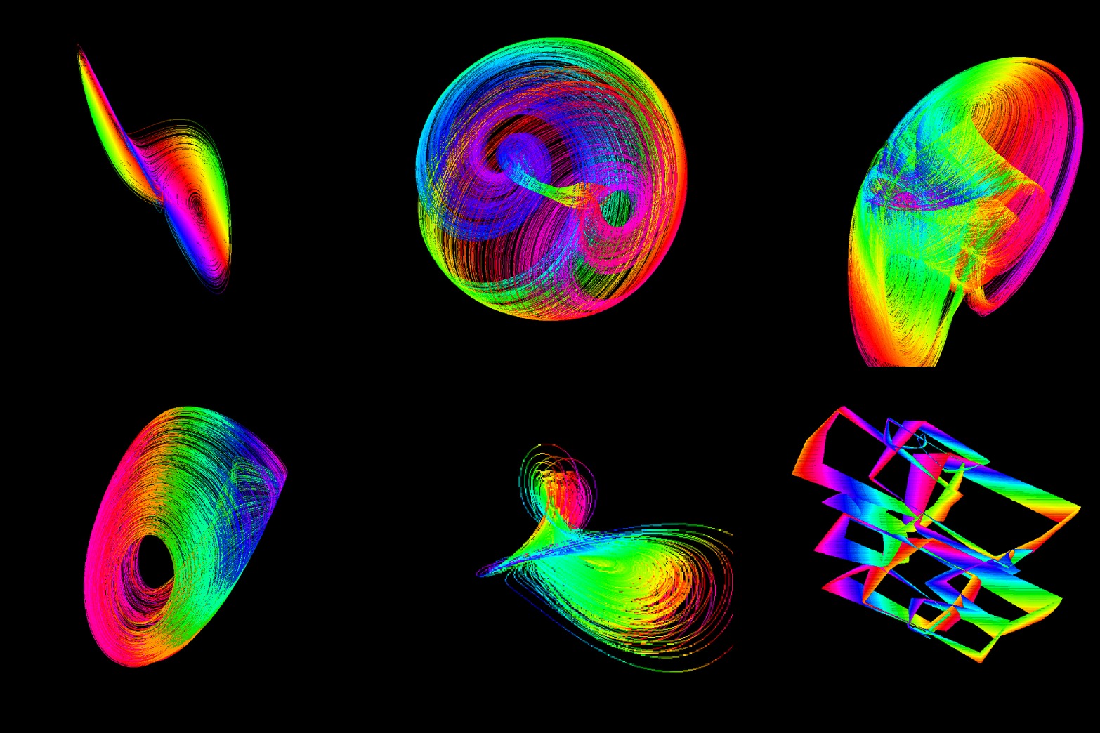


| FVF Wobbulator bank | XY oscilloscope |
|---|---|
 |
 |
Per-model animations, contact sheets and the chaos-monkey jam sessions: docs/gallery.md.
Aizawa mandalas. Seen end-on, the Aizawa attractor closes into a petaled
mandala, and its trail rainbow can be made to stand still, or to repeat as
harmonics: several rings outward, a wheel around, or a spiral. How these were
found, and the full table:
docs/aizawa-harmonics.md. On a local
chaosrack serve, the same links work with http://127.0.0.1:8080/ in place
of the site.
- 7 petals, 1 ring
- 7 petals, 2 rings outward
- 7 petals, 1 rainbow around (a color wheel)
- 7 petals, spiral
- 5 petals, 3 rings
- 3 petals, 3 rings
- 8 petals, 2 rings
- Lines still, colors flowing (one color cycle every 5 s)
- Lines moving, colors standing: the turns per loop are set to a golden-ratio value, so the orbit never closes, and the petals keep turning while the color rings hold
The first three found, with f above 0, where the orbit locks without fine tuning: one, two, three.
| source | |
|---|---|
| microphone | the default without --audio; getUserMedia, 1024-frame buffers (21 ms at 48 kHz) |
| generators | synthesized in the page, no buffer |
| system audio | chaosrack serve --audio: the PulseAudio/PipeWire monitor, as float32 over WebSocket, or WebTransport datagrams (?audio=wt) on lossy links |
?audio=mic and ?audio=ws force a source. The wire format and the
spectrogram engine are audioprism-go's.
A model of a 1984 frequency→voltage→frequency converter with a ring
modulator (bunkerofdoom.com): it tracks the input's
pitch, rescales it into a new carrier, and ring- or AM-modulates the input with
it. chaosrack serve --audio --wobbulate (or the route switch) routes all
system audio through it and plays the result on the speakers without feedback.
Signal path, routing and the hardware: docs/fvf.md.
The UI is tested in a real browser over the Chrome DevTools Protocol
(0magnet/cdp), by chaosrack uitool:
| subcommand | |
|---|---|
monkey |
seeded random-input fuzzer; invariants: no JS errors, no NaN readouts, panel recoverable, main thread alive |
golden |
fixed states: render sanity, permalink round-trip, golden images |
sweep |
every model and switch in order, with the monkey's invariants (make sweep) |
lint |
panel faults (overflow, overlap, centering, tooltips) by address (make lint-panel) |
layout · html · css |
geometry invariants · DOM validity · unused and conflicting CSS |
modules · portraits · shots · gifs |
capture the module reference, model images, hero/contact sheets, animations |
readme · site |
regenerate this file's generated sections · the model pages (--check to verify) |
catalog |
capture the native rack's panel |
demo |
recorded chaos-monkey performances |
spec |
WAV → spectrogram PNG through the app's pipeline |
They attach to a Chromium/Brave tab on --remote-debugging-port 9222, or run
their own headless browser with -headless -serve <binary>.
make test-wasm runs the js/wasm tests under Node with a fake DOM. Native tests
cover the pure logic and the chaos guard. make lint runs golangci-lint twice,
natively and under GOOS=js GOARCH=wasm. CI runs tests, both lint passes, a
wasm compile gate and a TinyGo build.
go build .                           # the host binary, with the wasm committed in assets/
GOOS=js GOARCH=wasm go build .       # the page alone
make check                           # lint, vet, test, readme-check
make help                            # every target
The host binary serves the wasm in assets/ with //go:embed. The committed
copies are rebuilt by CI after each push, so a binary built from a changed
checkout serves the old page until that lands. To serve your own changes,
build the wasm first, then the binary:
make wasm          # assets/gowasm/chaosrack.wasm (standard Go)
go install .       # or: go build .
chaosrack serve --audio
make tinywasm (needs TinyGo; slow), make metersworker (the analyzers' Web
Worker) and make wasms (all three) build the others. Leave the rebuilt
assets uncommitted — CI owns them:
git checkout assets/gowasm/chaosrack.wasm assets/gowasm/built-from.txt
make pages writes the deployed index.html pages, and make onefile the
single-file build (SERVERLESS.md).
The repository root is one program: main.go on a host, main_js.go in the
page. commands/ assembles the chaosrack command; assets/ holds the
embedded wasm and templates; pkg/ holds about 45 packages, chiefly
attractor (the app and panel), server, dynamics (the models' math),
meters, audiosrc, scope, rackspec, racklayout, racksurface,
rackhost (the native rack), preset, equation and stlmodels.
manual/ is the help text the tooltips and Info window show.
Browser attractor visualizers and audio tools:
- ibiblio e-notes — Lorenz / Rössler (WebGL, incl. GPU 1M-point)
- Harvard/Knill — animated Lorenz
- daybarr/lorenz-webgl
- Simulations4All — Lorenz with σ/ρ/β sliders
- KinnyTools — audio-reactive Lorenz
- jujiplay — interactive Rössler
- Shashank Tomar — Strange Attractors — fourteen systems as GPU particle systems; chaosrack's Arneodo, Chen–Lee, Dequan Li, Three-Scroll, Wang–Sun, Lorenz Mod 2 and Simone come from its catalog (discussion)
- libpd-wasm — Pure Data in an AudioWorklet
- SuperSonic — SuperCollider's scsynth in WebAssembly
- The Analog Computer Museum's library — manuals of EAI, Telefunken, Dornier and other analog computers
- Reconfigurable Analog Computers — digitally reconfigured analog computers as co-processors
- GitHub
strange-attractorstopic
Instrument panels and controls in the browser:
- webaudio-controls (demo) — knob, slider, switch and keyboard web components
- input-knobs —
<input>elements styled as knobs and switches - precision-inputs and NexusUI — knob, dial and matrix widgets
- iO-808 — a TR-808 in Web Audio
- Ableton Learning Synths — a guided synth tour
- Audiotool — hardware-style devices patched with cables
- Cardinal (VCV Rack in WebAssembly), Patchcab, DreamRack — Eurorack-style racks
- woscope — WebGL XY oscilloscope
Made with goda:
# GOOS=js: the import edges of a wasm program live in js/wasm-tagged
# files and are invisible to a host-context run
GOOS=js GOARCH=wasm go run github.com/loov/goda@latest graph github.com/0magnet/chaosrack/... | dot -Tsvg -o docs/chaosrack-goda-graph.svg

Made with gocloc (excludes vendor/, node_modules/, .git/):
gocloc --not-match-d='(vendor|node_modules|\.git)' .
-------------------------------------------------------------------------------
Language                     files          blank        comment           code
-------------------------------------------------------------------------------
Go                             614           8691          31925          81751
HTML                            87            684            417          11505
Markdown                        15           2292            706           4724
JSON                             4              0              0           3933
JavaScript                       6            199            287           2103
CSS                              1             98           1039            808
Makefile                         1             34             59            249
YAML                             1              0             19            149
Bourne Shell                     3             19             63             85
XML                              1              0              0             84
BASH                             1              8             25             79
Plain Text                       2              1              0              4
-------------------------------------------------------------------------------
TOTAL                          736          12026          34540         105474
-------------------------------------------------------------------------------